REVIEW 3 major objections 5 minor 15 references
Thickness-aware E(3)-Equivariant 3D Mesh Neural Networks
T0 review · 3 major / 5 minor · reviewed 2026-08-07 · deepseek-v4-flash
Pith's one-line read By adding one gated edge per node to its pair on the opposite face, T-EMNN predicts node-level 3D deformation on real industrial parts more accurately than surface-only mesh networks while keeping the low cost of a surface mesh.
desk verdict Useful thickness-aware message passing undermined by a flawed E(3)-invariance proof. read the letter →
The pith
A machine-rendered reading of the paper's core claim, the machinery that carries it, and where it could break.
The reading
What carries the argument
The load-bearing devices are the thickness edge and the data-driven coordinate system. A thickness edge connects a node vi to T(vi), the nearest node found by projecting a ray along the inward normal onto the opposing surface; its feature is the pair [t(vi), n_i·n_T], where t(vi) is the Euclidean distance between the paired nodes and the dot product measures normal alignment. Message passing along the edge is multiplied by the activation I_i = 1/(1 + exp(α(t(vi) − τ))) with α = 3, so edges below the learnable threshold τ pass nearly full weight and edges above it are masked, and this is what separates thickness from width. The coordinate system works by subtracting the center of mass, computing the PCA basis of the centered point cloud as the rotation matrix, flipping each axis to align with v = x_cm − x_bbox, and transforming every coordinate into that frame; the same stored rotation and center transform predictions back, which gives E(3)-equivariance.
What would settle it
Take a mesh with an n-fold rotational symmetry axis, such as a long cylinder or a regular prism, apply a rotation by 360/n degrees, and recompute x_inv via the paper's four steps; if the covariance matrix has repeated eigenvalues, the principal axes are not unique, and the resulting x_inv for corresponding nodes will differ, showing the claimed E(3)-invariance fails. An even simpler check uses a cube: for a uniformly sampled cube, the center of mass equals the bounding-box center, so the reference vector v in Eq. 5 is zero, the sign rule is undefined, and rotating the cube by any angle that permutes the principal axes will change the computed coordinates.
Extended reading notes
Core claim
The central claim is that thickness is not a side detail of mesh geometry but a first-class interaction: nodes on opposite faces of a solid are so tightly coupled that their deformations are far more correlated than any radius-based neighborhood, and modeling that coupling directly improves prediction. The paper demonstrates the correlation empirically and then shows that a single learned edge per node—connecting each node to the closest node on the opposing surface—is enough to exploit it, provided the edge is gated by a learnable thickness threshold so that pairs measuring 'width' rather than 'thickness' are filtered out. Equally central is the claim that raw spatial coordinates can be fed into an E(3)-equivariant network without expensive spherical harmonics: centering the mesh, taking PCA principal axes as a rotation, and fixing axis signs with a bounding-box reference yields a coordinate frame that is invariant to rotation, translation, and reflection, and the stored rotation and center make the decoder's output equivariant. The paper backs these claims with a real-world injection-molding dataset and reports that the full model outperforms all baselines on node-level 3D deformation while adding only a small computational overhead.
Load-bearing premise
The data-driven coordinate system is only E(3)-invariant if the shape's principal axes are uniquely determined and the sign rule resolves their direction; for rotationally symmetric shapes the PCA eigenspace is degenerate and the sign can stay ambiguous, in which case the rotation of the object can change the computed invariant coordinates.
Editorial extensions
If this is right
- Adding thickness edges improves RMSE and R2 for node-level 3D deformation prediction on a real industrial dataset, and the gain holds when test inputs are randomly rotated, because the data-driven coordinate frame keeps spatial features aligned.
- The learned threshold τ converges to a stable value (~5.68) across seeds and matches the best fixed-threshold sweep; removing thickness edges or setting the threshold too high (admitting width pairs) degrades performance.
- Plugging the same thickness edges and thickness processor into MGN, EGNN, and EMNN improves all three baselines, so the mechanism is a plug-in, not a redesign.
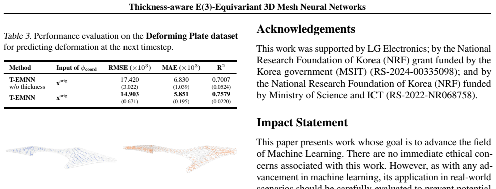
- On the Deforming Plate dynamics benchmark, thickness edges also improve next-timestep deformation prediction, showing the idea carries over from static analysis to time-dependent simulation.
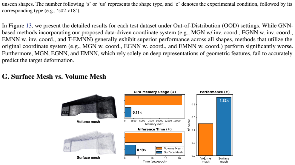
- The approach keeps the computational profile of a surface mesh: T-EMNN trains at about 20 iterations per second and uses roughly 3.7 GB GPU memory, far below EMNN's 7.3 GB.
Reading between the lines
- A testable extension is to replace the single scalar threshold with per-region or per-node thresholds, since real parts can have locally varying thickness; the paper's global τ may under-use thin regions or over-include thick ones.
- The thickness-edge idea is really a cheap way to add one specific long-range interaction, so it could be adapted to other paired physical couplings (contact pairs, symmetry planes, boundary layers) where surface-only message passing would need many hops to connect the two sides.
- The PCA coordinate frame's equivariance is hostage to the uniqueness of principal axes; for shapes with rotational symmetry the covariance eigenspace is degenerate, so a robust variant might predict jointly from all equivalent principal-axis choices or average invariant features, though that would change the architecture rather than the proof.
- Because the paper computes thickness pairs once per mesh and keeps them fixed over time in the dynamic experiment, a natural stress test is whether recomputing pairs as the mesh deforms changes predictions; if it does, the frozen-pair assumption is doing some of the work.
Editorial analysis
A structured set of objections, weighed in public.
Referee Report
Summary. This paper proposes T-EMNN, a mesh-based graph neural network for predicting node-level 3D deformation of objects with thickness. Two main components are introduced: (i) thickness edges that connect each surface node to a paired node on the opposing surface, with a learnable threshold and sigmoid activation to retain only 'true thickness' pairs; and (ii) a data-driven coordinate system built from the PCA of the shape's point cloud, intended to give E(3)-invariant spatial coordinates. The method is evaluated on a real-world injection-molding dataset and the Deforming Plate benchmark, reporting improved RMSE/MAE/R² over MGN, EGNN, and EMNN baselines, including under randomly rotated test inputs.
Significance. If the E(3)-invariance guarantee held, the data-driven coordinate system would be an attractive low-cost way to inject global spatial information into equivariant mesh networks, and the thickness-edge message passing is a simple, well-motivated mechanism for capturing through-thickness correlations that surface-only meshes miss. The experimental study is unusually careful: Table 1 separates the effects of spatial information and thickness edges, Fig. 6 validates the learned threshold by scanning fixed thresholds, Fig. 8 shows thickness edges help all baselines, and Table 4 documents computational cost. The main weakness is that the central theoretical claim--E(3)-invariance of the PCA-based coordinates--is not actually proved and, as stated, is false; this must be corrected or the claims substantially weakened before the contribution is complete.
major comments (3)
- [Sec. 4.1, Step 3 / Appendix H] The sign-alignment rule in Eq. (5) is not rotation-equivariant, so the claimed E(3)-invariance of x_inv does not hold even for generic non-degenerate shapes. The reference vector v = x_cm - x_bbox depends on the axis-aligned bounding box, and the componentwise min and max operations do not commute with rotations: under a rotation Q, v' != Q v in general. A concrete 2D example is X = {(0,0),(2,0),(0,2),(3,1)}; rotating the cloud by 30 degrees changes the sign of both PCA axes relative to the unrotated aligned frame, giving x_inv' = -x_inv. The proof in Appendix H explicitly states 'we assume that the signs of the basis vectors are already aligned,' which is precisely the step that fails, and Eq. (25) also uses an invalid matrix product (the covariance of the rotated data should be Q C_X Q^T, not C_X). Because x_inv is an input to the spatial encoder (Eq. 10) and decoder (Eq. 19), a sign flip changes the network's inputs and cannot be canceled by the inverse rotation unless the network is sign-equivariant, which is not the case for an MLP. Please replace Eq. (5) with a reference vector that transforms as a vector under E(3) (e.g., based on the farthest point from the center of mass) or substantially weaken the invariance/equivariance claims.
- [Sec. 3.3, Eq. (1)] The scalar d ('ray projection distance') is never defined or specified anywhere in the manuscript. Since T(v_i) is the argmin of ||x_j - (x_i - d·n_i)||, the selected thickness pair depends on d: as d approaches 0 the pair is the closest node on the opposite side, while as d grows large it approaches the node with the most negative projection along n_i. No value, tuning procedure, or default is reported in the experiments (Section 5) or the appendix, so the thickness-edge construction is not reproducible and the reported numbers cannot be independently checked. Please report d or justify that the results are insensitive to it over a wide range.
- [Sec. 4.2.4, inverse transformation] The final deformation is computed as p_orig_i = R·p_inv_i + x_cm. If p_inv_i is a deformation (displacement) vector predicted in the invariant coordinate system, the translation x_cm should not be added; displacements are vectors and transform under rotation only. Adding x_cm would make the prediction depend on the global position of the shape and is inconsistent with the stated task of predicting node-level deformation. Equation (8) is the correct inverse mapping for absolute coordinates, not for displacements. Please clarify whether the network predicts absolute deformed positions or displacements and correct the formula, or confirm that the reported experiments use R·p_inv_i and the equation is a typo.
minor comments (5)
- [Sec. 3.3, Eq. (1)] The strict inequality (x_j - x_i)·n_i < 0 may leave T(v_i) undefined if no node lies strictly on the opposite side; please state the fallback (e.g., ignore the thickness edge for that node).
- [Sec. 4.2.3, Eq. (15)] The sigmoid activation I_i is continuous, so edges with t(v_i) > tau are not actually excluded, only down-weighted; the text later says such edges are 'filtered out.' Clarify whether hard masking is applied at test time or whether the description is only approximate.
- [Table 4] Table 4 lists 'MLP' twice with identical input column '-'; presumably the second row should specify a coordinate input (x_orig or x_inv).
- [Appendix H, Eqs. (24)-(25)] The notation QX is dimensionally inconsistent when X is an N x 3 matrix; the covariance of rotated data should be expressed as Q C_X Q^T (or the matrix dimensions must be stated explicitly). This makes the derivation hard to follow.
- [Sec. 5.4.3] The dynamic experiment uses the original coordinate system because the data-driven coordinate system is 'designed for static analysis'; this is unexplained, since the coordinate transformation itself does not depend on time, and it weakens the comparison with the static results.
Circularity Check
No significant circularity found: the coordinate transform and thickness processor are derived from input geometry, and the ablations are sensitivity checks, not construction-level fits.
full rationale
The central derivation chain is self-contained. The data-driven coordinate system (Sec. 4.1) is constructed purely from input vertex positions: centering (Eqs. 3-4), PCA axes, sign alignment via the bounding-box reference vector (Eq. 5), and projection (Eq. 7). The target deformation enters only through the training loss; it is never used to define x_inv, R, or the thickness pairs. The E(3)-invariance proof (App. H) is a direct calculation for that construction; it contains an explicit unresolved case, namely "For the proof, we assume that the signs of the basis vectors are already aligned," which is a correctness/robustness gap for symmetric or adversarially rotated shapes, not a circular reduction. The thickness processor is likewise non-circular: T(v_i) and t(v_i) are geometric functions of the mesh (Eqs. 1-2), the threshold tau is a learned model parameter, and the fixed-threshold scan (Fig. 6) is a sensitivity/ablation check, not a prediction forced by construction. The only self-citation (Yu et al. 2023, which includes co-authors Lee and Park) appears in the related-work list of hierarchical pooling methods and is not load-bearing for any claim. No equation reduces to its own input, and no fitted parameter is renamed as a prediction; the paper's flagged limitation is a correctness concern, not circularity.
Assumptions & free parameters
free parameters (3)
- Thickness threshold tau =
5.68
- alpha (scaling factor) =
3
- d (ray projection distance) =
not reported
assumptions (3)
- domain assumption The point cloud used for PCA has non-degenerate principal components and sign alignment always succeeds.
- domain assumption The mesh is water-tight and has consistently oriented outward normals.
- domain assumption The nearest qualifying node along the inward normal is the physically meaningful opposing point.
invented entities (3)
-
Thickness edge
-
Thickness node pair
-
Data-driven coordinate system
Cite this review
Pith. "Pith review of Thickness-aware E(3)-Equivariant 3D Mesh Neural Networks." pith.science (2026). https://pith.science/paper/UZIS4DVA
@misc{pith2026250521572,
  author       = {Pith},
  title        = {Pith review of: Thickness-aware E(3)-Equivariant 3D Mesh Neural Networks},
  year         = {2026},
  howpublished = {\url{https://pith.science/paper/UZIS4DVA}},
  note         = {Machine review of arXiv:2505.21572}
}
read the original abstract
Mesh-based 3D static analysis methods have recently emerged as efficient alternatives to traditional computational numerical solvers, significantly reducing computational costs and runtime for various physics-based analyses. However, these methods primarily focus on surface topology and geometry, often overlooking the inherent thickness of real-world 3D objects, which exhibits high correlations and similar behavior between opposing surfaces. This limitation arises from the disconnected nature of these surfaces and the absence of internal edge connections within the mesh. In this work, we propose a novel framework, the Thickness-aware E(3)-Equivariant 3D Mesh Neural Network (T-EMNN), that effectively integrates the thickness of 3D objects while maintaining the computational efficiency of surface meshes. Additionally, we introduce data-driven coordinates that encode spatial information while preserving E(3)-equivariance or invariance properties, ensuring consistent and robust analysis. Evaluations on a real-world industrial dataset demonstrate the superior performance of T-EMNN in accurately predicting node-level 3D deformations, effectively capturing thickness effects while maintaining computational efficiency.
Figures


Figures from the paper (11 more)






Reference graph
Works this paper leans on
-
[1]
Alon, U. and Yahav, E. On the bottleneck of graph neural networks and its practical implications.arXiv preprint arXiv:2006.05205,
arXiv 2006
- [5]
-
[6]
Directional message passing for molecular graphs.arXiv preprint arXiv:2003.03123,
Gasteiger, J., Groß, J., and G ¨unnemann, S. Directional message passing for molecular graphs.arXiv preprint arXiv:2003.03123,
arXiv 2003
-
[8]
Janny, S., Beneteau, A., Nadri, M., Digne, J., Thome, N., and Wolf, C. Eagle: Large-scale learning of turbulent fluid dynamics with mesh transformers.arXiv preprint arXiv:2302.10803,
-
[14]
Comparisons between volume mesh and surface mesh. The methods used for comparison are based on the MGN framework with coordinate embeddings from our proposed coordinate system. GPU memory usage represents the average GPU consumption across the test dataset, and inference time reflects the total time required to process the test dataset. Mesh representatio...
work page 2020
-
[1991]
Constraint-based graph network simulator
Rubanova, Y ., Sanchez-Gonzalez, A., Pfaff, T., and Battaglia, P. Constraint-based graph network simulator. arXiv preprint arXiv:2112.09161,
-
[2007]
Pfaff, T., Fortunato, M., Sanchez-Gonzalez, A., and Battaglia, P. W. Learning mesh-based simulation with graph networks.arXiv preprint arXiv:2010.03409,
arXiv 2010
-
[2008]
Pre- dicting physics in mesh-reduced space with temporal attention.arXiv preprint arXiv:2201.09113,
Han, X., Gao, H., Pfaff, T., Wang, J.-X., and Liu, L.-P. Pre- dicting physics in mesh-reduced space with temporal attention.arXiv preprint arXiv:2201.09113,
Show all 15 references
-
[2010]
Generalized beam theory applied to shear stiff- ness.International Journal of Solids and Structures, 27 (15):1955–1967,
Renton, J. Generalized beam theory applied to shear stiff- ness.International Journal of Solids and Structures, 27 (15):1955–1967,
1955
-
[2018]
Learning flexible body collision dynamics with hier- archical contact mesh transformer.arXiv preprint arXiv:2312.12467,
Yu, Y .-Y ., Choi, J., Cho, W., Lee, K., Kim, N., Chang, K., Woo, C.-S., Kim, I., Lee, S.-W., Yang, J.-Y ., et al. Learning flexible body collision dynamics with hier- archical contact mesh transformer.arXiv preprint arXiv:2312.12467,
-
[2019]
Multiscale meshgraphnets.arXiv preprint arXiv:2210.00612,
Fortunato, M., Pfaff, T., Wirnsberger, P., Pritzel, A., and Battaglia, P. Multiscale meshgraphnets.arXiv preprint arXiv:2210.00612,
-
[2020]
Neural operator: Graph kernel network for partial differential equations
Anandkumar, A., Azizzadenesheli, K., Bhattacharya, K., Kovachki, N., Li, Z., Liu, B., and Stuart, A. Neural operator: Graph kernel network for partial differential equations. InICLR 2020 Workshop on Integration of Deep Neural Models and Differential Equations,
2020
-
[2021]
Suk, J., de Haan, P., Lippe, P., Brune, C., and Wolterink, J. M. Equivariant graph neural networks as surrogate for computational fluid dynamics in 3d artery models. In Fourth workshop on machine learning and the physical sciences (NeurIPS 2021),
2021
-
[2022]
J., and Welling, M
Brandstetter, J., Hesselink, R., van der Pol, E., Bekkers, E. J., and Welling, M. Geometric and physical quantities improve e (3) equivariant message passing.arXiv preprint arXiv:2110.02905,
-
[2023]
Deeper insights into graph convolutional networks for semi-supervised learning
Li, Q., Han, Z., and Wu, X.-M. Deeper insights into graph convolutional networks for semi-supervised learning. In Proceedings of the AAAI conference on artificial intelli- gence, volume 32, 2018a. Li, Y ., Wu, J., Tedrake, R., Tenenbaum, J. B., and Torralba, A. Learning partic...
Reviewed August 7, 2026 · model on record in the stance chip above.
Discussion (0). Sign in to comment.