Statistical microlocal analysis in two-dimensional X-ray CT

Alexander Katsevich; Anuj Abhishek; James W. Webber

REVIEW 3 major objections 4 minor 50 references

Statistical microlocal analysis in two-dimensional X-ray CT

T0 review · 3 major / 4 minor · reviewed 2026-08-07 · deepseek-v4-flash

Challenge this review Re-run · record.json Download PDF Read on arXiv ↗

Pith's one-line read For CT images reconstructed from noisy, finite-step data, edge detectability is a computable probability rather than a deterministic yes-or-no property.

desk verdict A genuinely new statistical take on microlocal edge detectability in CT, with a solid main theorem and good simulations, but a load-bearing numerical inconsistency in the covariance that needs to be fixed. read the letter →

arxiv 2506.05113 v3 pith:J2ZTFIS7 submitted 2025-06-05 math.ST math.FAstat.TH

Anuj Abhishek , Alexander Katsevich , James W. Webber This is my paper

classification math.STmath.FAstat.TH MSC 62F0362H1562M4044A1265R10

keywords statisticalmicrolocalanalysisedgedetectionX-raycomputedtomographyRadontransformGaussianrandomfieldlikelihood-ratiotestnoncentralchi-squareddistributionuncertaintyquantification

verification ladder T0 review T1 audit T2 compute T3 formal

The pith

A machine-rendered reading of the paper's core claim, the machinery that carries it, and where it could break.

The reading

The paper introduces Statistical Microlocal Analysis, a way to turn the question “is there an edge at this point in a CT image?” into a statistical test. Its claim is that, at the finest scale compatible with the data, a weighted local integral of the reconstructed image is a bivariate Gaussian: zero-mean when no edge is present, and shifted by a vector proportional to the edge’s jump and normal to the edge when one is. From that distribution the paper derives the power of the optimal likelihood-ratio test, so edge detectability becomes a computed probability that depends on the noise level, the sampling step, and the jump size. If the claim holds, practitioners can predict how likely a feature is to be seen or missed, and can draw explicit confidence regions for edge magnitude and direction.

What carries the argument

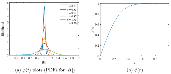
The argument rides on three objects. The first is the discrete transition behavior (DTB) function $f_T(t)=\int_{-\infty}^{t}\varphi(s)\,ds - 1/2$, a smoothed unit step describing how a jump in the object is rounded by finite sampling. The second is the zero-mean Gaussian random field $N^{\mathrm{rec}}$ that limits the reconstruction noise, with stationary covariance $C(\check{x})=(\kappa/4\pi)^2\int_0^{2\pi}\sigma^2(\alpha,\vec\alpha\cdot x_0)(\varphi'\star\varphi')(\vec\alpha\cdot\check{x})\,d\alpha$. The third, which carries the statistical test, is the vector $F$: the first moment of the reconstruction over an $O(\epsilon)$-sized disk. The edge response $f_T$ is nearly constant along the edge while the Gaussian random field oscillates, so the disk integral averages away noise without cancelling the edge signal; that separation is why $F$ distinguishes the null from the alternative and why $E(F)=H$.

What would settle it

Reconstruct a fixed disk phantom from many independent noise draws at several step sizes (for example $\epsilon=0.02, 0.01, 0.007, 0.003$), compute $F$ from (4.1) each time, and compare the empirical covariance and rejection rates against $\hat C$ and $1-\Upsilon_1(-2\ln\alpha)$; if the empirical power does not approach the predicted curve as $\epsilon$ shrinks, the Gaussian approximation (2.11) is not the right limit. A second check is to move $x_0$ to a point where $\kappa|x_0|$ is rational, which should break Assumption 2.5 and change the distribution.

Watch

Extended reading notes

Core claim

The central discovery is that noise and finite sampling do not merely blur edge detectability; they give it a computable distribution. For a point $x_0$ satisfying Assumption 2.5, the vector $F = \int_{B_\rho(0)} \check{y}\, f^{\mathrm{rec}}(x_0+\epsilon\check{y})\,d\check{y}$ obeys $H_0: F \sim N(0,\hat C)$ (no edge) versus $H_1: F \sim N(H,\hat C)$ (edge), where $H$ is normal to the edge and $|H|$ is proportional to the jump $\Delta f$. The likelihood-ratio test that rejects $H_0$ when $\|F\|^2_{\hat C^{-1}} > -2\ln\alpha$ has power $1-\Upsilon_1(-2\ln\alpha)$, with $\Upsilon_1$ the CDF of a noncentral chi-squared variable with noncentrality parameter $\|H\|^2_{\hat C^{-1}}$. Since $E(F)=H$, the vector $F$ is an unbiased statistical estimate of the edge’s conormal vector, and a confidence region for $H$ at level $1-\alpha$ is the ellipse $\{H : \|F-H\|_{\hat C^{-1}} \le (-2\ln\alpha)^{1/2}\}$.

Load-bearing premise

The load-bearing premise is that, in a window of size comparable to the sampling step, the noisy reconstruction is a known smoothed step plus a zero-mean Gaussian random field with the covariance in (2.10); this is proven only in the limit as the step size goes to zero, and the paper applies it at finite step sizes such as $\epsilon=0.007$.

Editorial extensions

If this is right

Edge presence at a fixed point in 2D CT can be reported as a power $1-\beta = 1-\Upsilon_1(-2\ln\alpha)$, computed from the noise level, sampling step, scanner ratio, and jump size via the noncentral chi-squared CDF.
For any chosen confidence level, the true edge vector $H$ lies in an ellipse centered at the observed $F$, and in the isotropic-noise case this is a circle; the paper’s simulation reports the predicted 95% coverage to two significant figures.
Uncertainty in direction and magnitude can be separated: marginal PDFs give statements such as “the edge direction is within $\pm 26^\circ$ of the true direction with 95% probability” at the simulated noise level.
The power of the test can be made arbitrarily close to 1 for a fixed signal-to-noise ratio by enlarging the window radius $\rho$, because the noncentrality parameter grows at least linearly in $\rho$.
The pointwise guarantee applies to one fixed point; when the same test is slid across a full image, neighboring windows are dependent, so the paper presents the macro-scale scan only as an illustration.

Reading between the lines

Editorial extensions of the paper, not claims the author makes directly.

My inference: the same construction should transfer to other generalized Radon transforms that admit a local edge-profile expansion and a Gaussian random-field noise limit, such as synthetic aperture radar or ultrasound, but the paper proves it only for 2D X-ray CT.
My inference: the Diophantine conditions on $\kappa|x_0|$ suggest that “bad” points where this quantity is rational may show measurably different, possibly non-Gaussian, local statistics; an experiment comparing rational and irrational values would probe how sharp those conditions are.
My inference: because $F$ is the first moment of the reconstruction over the disk, other weights (such as higher-order moments or wavelet-type kernels) would give different power–direction-resolution trade-offs; the paper fixes the weight $\check{y}$ and does not optimize over kernels.
My inference: the finite-$\epsilon$ error in the local approximation could itself be estimated by comparing predicted and observed distributions across a sequence of step sizes; if the error decays like $O(\epsilon)$, the method could be extended to give a discretization-bias-corrected confidence statement.

Share X Bluesky LinkedIn Reddit HN

Editorial analysis

A structured set of objections, weighed in public.

Desk editor's note, referee report, and a circularity audit.

Desk Editor's Note

read the letter

The paper does something new. It turns the classical microlocal question of edge detectability in CT from a noiseless, continuous-data statement into a concrete hypothesis test with explicit power for noisy, finite-step 2D data. That is a useful capability, and the SMA framework is a real contribution, not just a relabeling of existing ideas.

The construction of the test statistic F as a weighted integral of the reconstruction over an O(epsilon) disk is the right move, and the use of the Gaussian random field covariance from the authors' prior work [1] to get its distribution is sound. Theorem 4.1 is short but correct given the local approximation (2.11), and the simulations are extensive: the null and shifted PDFs match predictions well, the ROC curves agree, and the 1D vs 2D power comparison is sensible. The authors are also honest about the scan-statistic caveat in Section 5.5 and about the grid-step-size issue.

The main problem is an internal inconsistency in Section 5.2. The predicted covariance is reported as diag(0.074, 0.074), but the text then states nu^2 = 0.14. The observed covariance is about 0.074, so the validation uses 0.074, while the direction-uncertainty calculation in Section 5.3 appears to use the 0.14 value. Since the test statistic, power, and confidence region all depend on C-hat, this is load-bearing rather than a harmless typo. It also explains the 26-degree predicted vs 20-degree observed mismatch in Section 5.3. The fix should be to use the consistent value (likely 0.074) and recalculate the direction spread.

A lesser issue: the reconstruction kernel phi is never specified, which hampers reproducibility of the numerical predictions. Also, the whole framework rests on the finite-epsilon accuracy of (2.11); the simulations suggest it works at epsilon=0.007, but the paper does not quantify the rate of convergence, so practitioners should be cautious when moving to larger step sizes.

This paper deserves a serious referee. The core idea is novel and the mathematical scaffolding, aside from the covariance inconsistency, is sound. The readers who will get value are researchers and practitioners in CT and statistical inverse problems. I would cite it after the covariance is corrected.

Referee Report

3 major / 4 minor

Summary. The paper introduces Statistical Microlocal Analysis (SMA) for 2D X-ray CT: given noisy, discretely sampled Radon data and a reconstruction at native scale epsilon, the authors define a random vector F obtained by weighted integration of the reconstruction over an O(epsilon) disk, and characterize its distribution using prior Local Reconstruction Analysis and Gaussian random field results. Under the null hypothesis of no edge, F is approximately Gaussian with zero mean and covariance C-hat; under an edge, F is approximately Gaussian with mean H proportional to the jump and the same covariance. The likelihood-ratio test statistic is ||F||^2_{C-hat^{-1}}, which is chi-square under H0 and noncentral chi-square under H1, yielding explicit power formulas. The authors also construct confidence regions for H and study uncertainty in edge direction and magnitude, and they validate the predictions against simulations of a disk phantom.

Significance. If the distributional and power results are correct, this is a genuinely useful extension of classical microlocal detectability conditions to noisy, finite-step data: it replaces the deterministic visibility criterion with a computable probability of detection, and it gives confidence regions for edge magnitude and direction. The paper's strengths include explicit, parameter-free formulas (no fitted constants in the central test), a proof of the 2D LRT theorem that is standard once the Gaussian approximation is granted, and simulation checks with large sample sizes. The authors are also appropriately candid about limitations, including the scanning-regime issue and the reliance on approximation (2.11). However, the validation contains an internal numerical inconsistency, and the 1D power formula (3.12) is not the correct normal tail probability as written; these issues block the numerical claims until corrected.

major comments (3)

[Section 5.2, Eq. (4.4) and Remark 2] The covariance is reported inconsistently. The text says 'using (4.4), we predict that G is normally distributed with mean zero and covariance C-hat = [[0.074,0],[0,0.074]]' and then 'Since sigma is a constant function, C-hat = nu^2 I_2, nu^2 = 0.14'. If the diagonal entries are 0.074, then nu^2 must equal 0.074, not 0.14. The observed covariance quoted immediately afterward, [[0.074,0],[0,0.075]], supports nu^2 = 0.074. This is load-bearing because Theorem 4.1, the rejection threshold r = nu sqrt(-2 ln alpha), the power formula (5.1), the confidence region (4.12), and the direction-uncertainty calculation in Section 5.3 (omega = 26 degrees versus observed about 20 degrees) all depend on C-hat through C-hat^{-1}. The numerical content of the validation is therefore not well-defined until this is corrected.
[Section 3.2, Eq. (3.12)] The displayed formula for the type II error is not correct as written. Under H1, F_u/gamma ~ N(m,1) with m = H_u/gamma, and the rejection region is |F_u|/gamma > sqrt(c_alpha). Hence beta = P(|N(m,1)| <= sqrt(c_alpha)) = Phi(sqrt(c_alpha)-m) - Phi(-sqrt(c_alpha)-m) = 0.5[erf((sqrt(c_alpha)-m)/sqrt(2)) + erf((sqrt(c_alpha)+m)/sqrt(2))]. The formula in (3.12) instead uses c_alpha inside the erf arguments and subtracts, which does not reduce to this normal tail probability. Since the predicted ROC and AUC in Section 5.1 are computed from (3.12), the 1D power predictions need to be recomputed with the correct expression and the comparison with the observed AUC re-examined.
[Theorem 4.1 and approximation (2.11)] Theorem 4.1 is stated as an exact distributional statement for fixed epsilon, but its proof relies on approximation (2.11), which combines the deterministic expansion (2.7) with weak convergence of the GRF from Theorem 2.6; no convergence rate or finite-epsilon error bound is supplied. The random vector F in (4.1) depends on epsilon through f^rec_{epsilon,eta}(x0+epsilon y), but this dependence is suppressed and the theorem gives no epsilon-quantified error. Please state Theorem 4.1 as an asymptotic result in the limit epsilon -> 0, or provide a quantified bound on the approximation error, and adjust the finite-epsilon validation claims accordingly. This is a formal gap rather than a fatal flaw, but it is load-bearing for the claimed power and confidence regions at finite epsilon.

minor comments (4)

[Sections 5.1 and 5.2] The notation 'eta ~ U(0,sigma)' is contradictory if the noise is said to have mean zero and standard deviation sigma; a zero-mean uniform distribution with standard deviation sigma would be U(-sqrt(3)sigma, sqrt(3)sigma). Please clarify the actual noise distribution used.
[Eq. (4.1)] In the definition F := integral_{B_rho(0)} y f^rec(y) dy, the arguments on the right are rescaled variables, so the notation should make explicit that f^rec(y) means f^rec_{epsilon,eta}(x0 + epsilon y); otherwise the integral appears to be over physical coordinates.
[After Eq. (4.3)] The sentence 'Thus, in the absence of noise, F = H' should be weakened to 'up to the O(epsilon) remainder in (2.7)', since the deterministic expansion is only asymptotic.
[Theorem 4.1 hypotheses] The statement assumes x0 satisfies Assumption 2.5 and then considers H0 with x0 not in S. Assumption 2.5(4)-(6) refer to the smooth singular support S at x0, so they are not meaningful when x0 is not on S. Please reformulate the hypotheses so that the null case is well defined, e.g., by stating that the same covariance formula is evaluated for a candidate point regardless of whether the edge is present.

Circularity Check

0 steps flagged · score 1.0 of 10

No circularity: Theorem 4.1 is a direct application of the authors' prior GRF limit theorem and standard likelihood-ratio theory, and the power claim is checked against independent simulations; the Section 5.2 C-hat versus nu^2 inconsistency is a correctness issue, not a circular step.

full rationale

The paper's central claim, Theorem 4.1, derives the distribution of the vector F from the Gaussian random field limit (Theorem 2.6, quoted from the authors' prior work [1]) and from the deterministic local reconstruction expansion (2.7, quoted from [16,20]). These two inputs are stated with explicit hypotheses (Assumptions 2.2, 2.3, 2.5), and neither input already contains the target conclusion that F is a bivariate Gaussian whose mean equals H. The Gaussianity of F then follows by linearity of the weighted integral and Proposition 6.1, and the test statistic, rejection threshold, and noncentral chi-squared power formula follow from the classical LRT fact that for F ~ N(H, C-hat) the quadratic form ||F||^2_{C-hat^{-1}} has chi-squared or noncentral chi-squared distribution. This is a derivation, not a restatement of an assumption: the covariance matrix C-hat is computed from the GRF covariance (2.10), and no parameter is fitted to the simulation output. The simulation studies are genuine external checks: full CT reconstructions with pseudorandom uniform noise are compared with the predicted Gaussian PDFs, ROC curves, AUC values, and confidence-region coverage; the paper reports observed values that match the predictions without tuning constants. The paper does rely heavily on the authors' own prior work, but that work is independent, parameter-free support with stated assumptions and does not assume the present result. The only serious defect found is internal: Section 5.2 states C-hat = diag(0.074, 0.074) and then says 'C-hat = nu^2 I_2, nu^2 = 0.14 (see Remark 2)', even though Remark 2 defines nu^2 as the diagonal entry of C-hat, so the stated numbers are mutually inconsistent. That ambiguity affects the numerical power, direction uncertainty, and confidence-region calculations, but it is a correctness/consistency problem rather than a circular reduction of the derivation to its own inputs. Under the required standard, no circular step is identifiable.

Assumptions & free parameters 2 free parameters · 7 assumptions · 0 invented entities

The paper's results depend on the local asymptotic characterization of the reconstruction (2.11), which is taken from the authors' prior work [1,16,20]. The assumptions on f, noise, kernel, and the Diophantine conditions at x0 are all needed for that characterization. Proposition 6.1 and the chi-squared properties are standard. No invented entities are introduced. The only hand-chosen tuning parameters are the window radius rho and the 1D weight kernel u.

free parameters (2)

window radius rho = 3 in simulations
Hand-chosen size of the O(epsilon) integration window. The power and covariance estimates depend on it; the theory allows any rho, but the paper does not provide a data-driven selection rule.
1D test kernel u(t) = chi_rho(t) t and chi_rho(t) sgn(t) in simulations
Hand-chosen weight function for the 1D statistic (3.7). The power depends on the choice, and the paper shows two options with similar performance but no optimality criterion.

assumptions (7)

domain assumption Assumption 2.1: f is a finite sum of smooth functions times characteristic functions of sets with piecewise smooth boundary.
Restricts to jump-type singularities, which is the setting of the theory. Invoked in Section 2.
domain assumption Assumption 2.2: noise has zero mean, variance sigma^2 Delta alpha, and bounded third moment.
Ensures weak convergence to a GRF with covariance (2.10). Invoked in Section 2.
domain assumption Assumption 2.3: interpolation kernel phi compactly supported, exact up to order 1, etc.
Needed for DTB and resolution analysis; exact kernel not specified in the paper, which hampers reproduction.
domain assumption Assumption 2.5: Diophantine conditions on kappa |x0|, curvature nonzero, etc.
Technical conditions for the asymptotic formulas (2.7) and Theorem 2.6 to hold; generic but unverifiable in practice.
domain assumption Theorem 2.6 from [1]: N^rec converges weakly to a GRF with covariance (2.10).
Relies on prior work by the same authors; the current paper's distributional claims inherit its validity.
standard math Proposition 6.1: linear functionals of a GRF are Gaussian with variance given by the double integral of the covariance.
Standard Gaussian random field fact, proved via partition approximation in the appendix.
standard math LRT facts: Z ~ chi^2_2 under H0 and noncentral chi^2_2 under H1.
Standard properties of multivariate normal quadratic forms, used in Theorems 3.1 and 4.1.

how reviews work

0 comments

Cite this review

Pith. "Pith review of Statistical microlocal analysis in two-dimensional X-ray CT." pith.science (2026). https://pith.science/paper/J2ZTFIS7

@misc{pith2026250605113,
  author       = {Pith},
  title        = {Pith review of: Statistical microlocal analysis in two-dimensional X-ray CT},
  year         = {2026},
  howpublished = {\url{https://pith.science/paper/J2ZTFIS7}},
  note         = {Machine review of arXiv:2506.05113}
}

abstract

In many imaging applications it is important to assess how well the edges of the original object, $f$, are resolved in an image, $f^\text{rec}$, reconstructed from the measured data, $g$. In this paper we consider the case of image reconstruction in 2D X-ray Computed Tomography (CT). Let $f$ be a function describing the object being scanned, and $g=Rf + \eta$ be the Radon transform data in $\mathbb{R}^2$ corrupted by noise, $\eta$, and sampled with step size $\sim\epsilon$. Conventional microlocal analysis provides conditions for edge detectability based on the scanner geometry in the case of continuous, noiseless data (when $\eta = 0$), but does not account for noise and finite sampling step size. We develop a novel technique called Statistical Microlocal Analysis (SMA), which uses a statistical hypothesis testing framework to determine if an image edge (singularity) of $f$ is detectable from $f^\text{rec}$, and we quantify edge detectability using the statistical power of the test. Our approach is based on the theory we developed in previous work, which provides a characterization of $f^\text{rec}$ in local $O(\epsilon)$-size neighborhoods when $\eta \neq 0$. We derive a statistical test for the presence and direction of an edge microlocally given the magnitude of $\eta$ and data sampling step size. Using the properties of the null distribution of the test, we quantify the uncertainty of the edge magnitude and direction. We validate our theory using simulations, which show strong agreement between our predictions and experimental observations. Our work is not only of practical value, but of theoretical value as well. SMA is a natural extension of classical microlocal analysis theory which accounts for practical measurement imperfections, such as noise and finite step size, at the highest possible resolution compatible with the data.

Figures

Figures reproduced from arXiv: 2506.05113 by the authors.

**Figure 1.** Illustration of the ROC curve. We begin by considering weighted integrals of the reconstructed image over a line segment. Select an odd, compactly supported function u ∈ L∞(R) and consider the quantity Fu = Z R u(t)fT (t)dt + Z R u(t)N rec(t)dt =: Hu + Gu, (3.7) where Nrec is the part of the reconstruction only from noise and fT is the deterministic part of f rec ϵ,η (the DTB function), see (2.8) and (2.11). Since u… view at source ↗

**Figure 2.** (a) Test phantom is a ball. The red horizontal line, which represents the edge detection [PITH_FULL_IMAGE:figures/full_fig_p015_2.png] view at source ↗

**Figure 3.** (A) and (B) - example Fu histograms and PDFs when u(t) = χρ(t)t. Recall that in the 1D case, the random variable Fu is proportional to the jump magnitude across a possible edge location. (C) - predicted and observed ROC curves. -1 -0.8 -0.6 -0.4 -0.2 0 0.2 0.4 0.6 0.8 1 -0.2 0 0.2 0.4 0.6 0.8 1 1.2 (a) AUC = 0.99, σ = 0.87 -1 -0.8 -0.6 -0.4 -0.2 0 0.2 0.4 0.6 0.8 1 -0.5 0 0.5 1 1.5 (b) AUC = 0.93, σ = 1.73 -1 -0.8 -… view at source ↗

Figures from the paper (10 more)

**Figure 4.** Figure 4: 1D line profiles (along {x2 = −0.1}) of reconstructions of the image phantom for varying σ. (a) Fu histograms -2 -1 0 1 2 -2 F u 0 0.2 0.4 0.6 0.8 1 pdf observed (null) predicted (null) observed (edge) predicted (edge) (b) prediction vs observed 0 0.2 0.4 0.6 0.8 1 0 0…

**Figure 5.** Figure 5: (A) and (B) - example Fu histograms and PDFs when u(t) = χρ(t)sgn(t). These plots are similar to the ones observed in [PITH_FULL_IMAGE:figures/full_fig_p016_5.png]

**Figure 6.** Figure 6: Local 1D line profiles of the reconstructions when [PITH_FULL_IMAGE:figures/full_fig_p017_6.png]

**Figure 7.** Figure 7: Deterministic part of the reconstruction. (a) - predicted local reconstruction of spherical [PITH_FULL_IMAGE:figures/full_fig_p018_7.png]

**Figure 8.** Figure 8: Predicted and observed PDFs of F. Top row - null distributions (F = G), in this case there is no edge and H = 0. Bottom row - shifted (edge) distributions (F = G + H). The right column shows 1D marginals of the PDFs (through the F1 axis). 18 [PITH_FULL_IMAGE:figures/f…

**Figure 9.** Figure 9: In (b) and (c) we show the PDF plots from figure [PITH_FULL_IMAGE:figures/full_fig_p019_9.png]

**Figure 10.** Figure 10: (a) - Computed observations, F (103 samples), when there is an edge present. The individual observations are marked by ‘x’. The observations are scaled by 1/|H| to reflect the true jump magnitude, i.e., 1 in this case. We also show the level sets, Bcα (H), of the pred…

**Figure 11.** Figure 11: (a) Polar graphs of φ(θ) for varying σ illustrating the probability of the edge occuring in a given direction. (b) Plot of ϕ(ω) for σ = √ 3. 5.4 Uncertainty in estimating the edge magnitude In a similar vein to the previous section, here we use our derived PDF for F t…

**Figure 12.** Figure 12: (a) Polar graphs of φ(t), the PDF for F, for varying σ. (b) Plot of ϕ(r). this section, we illustrate how we can employ F to detect edges on the full image (macro) scale. In this example, a globally reconstructed image is fixed, and we slide the window x0 + ϵBρ(0) acr…

**Figure 13.** Figure 13: (a) Noisy reconstruction of image phantom on full image scale. (b) and (c) Map of [PITH_FULL_IMAGE:figures/full_fig_p023_13.png]

Discussion (0). Sign in to comment.

Reference graph

Works this paper leans on

50 extracted references · 50 canonical work pages

[1]

2.σ 2(α, ⃗ α·x0)̸= 0for allαin some open setΩ⊂[0,2π]

The quantityκ|x 0|is irrational and of some finite typeν. 2.σ 2(α, ⃗ α·x0)̸= 0for allαin some open setΩ⊂[0,2π]. 3.|x 0|< P

work page
[2]

This shows that the desired confidence region is the ellipsoidE r(F), wherer=−2 lnα

Thusris found from the transformed equationP(∥v∥ 2 ≤r) = 1−α, which gives the familiarr= Υ −1 0 (1−α) =−2 lnα. This shows that the desired confidence region is the ellipsoidE r(F), wherer=−2 lnα. For the convenience of the reader, we have just derived the confidence region from first principles. An easier and more direct approach, which gives the exact sa...

work page
[3]

For example, settingα= 0.05 givesω= 26 ◦

This plot illustrates 20 how likely it is for the estimated edge directionF/|F|to deviate from the true directionH/|H|by no more than a given angle. For example, settingα= 0.05 givesω= 26 ◦. Thus the direction of the edge does not deviate by more than 26 ◦ from ⃗Θ0 with 95% probability. Using the 10 4 samples we generated to calculate theH+Ghistogram in t...

work page
[4]

The curvature ofSatx 0 is not zero

work page
[5]

The quantityκx 0 · ⃗Θ⊥ 0 is irrational, where ⃗Θ0 ∈S 1 is normal toSatx 0

work page
[6]

6 The asymptotic behaviour off rec ϵ (x) in a small neighborhood ofx 0 asϵ→0, is well understood from the theory of local reconstruction analysis (LRA), see e.g

The line{x∈R 2 : (x−x 0)· ⃗Θ0 = 0}is not tangent toSat any point where the curvature of Sis zero. 6 The asymptotic behaviour off rec ϵ (x) in a small neighborhood ofx 0 asϵ→0, is well understood from the theory of local reconstruction analysis (LRA), see e.g. [16, 17, 19, 18, 20]. Let ∆f(x 0) := lim t→0+ f(x 0 +t ⃗Θ0)−f(x 0 −t ⃗Θ0) (2.6) be the value of t...

work page
[7]

Felea, R

R. Felea, R. Gaburro, and C. J. Nolan. Microlocal analysis of sar imaging of a dynamic reflectivity function.SIAM Journal on Mathematical Analysis, 45(5):2767–2789, 2013

work page 2013
[8]

All other parameters, e.g.,ϵare kept the same as before

This equates to the ratio of theL 2 norms of the noise and the nonrandom signal in the CT data being 15% (i.e., NSR= 15%). All other parameters, e.g.,ϵare kept the same as before. We see in figure 13c that|F|highlights the true edges well and the edge map can be recovered accurately as in figure 13e using a simple threshold. We show|F|with no noise in fig...

work page

Show all 50 references

[9]

Eugene Katsevich, Statistics Department, University of Pennsylvania, for helpful discussions about confidence regions

AK is thankful to Prof. Eugene Katsevich, Statistics Department, University of Pennsylvania, for helpful discussions about confidence regions. 24 References Cited
[10]

Abhishek, A

A. Abhishek, A. Katsevich, and J. W. Webber. Local reconstruction analysis of inverting the Radon transform in the plane from noisy discrete data.SIAM Journal on Imaging Sciences, 18(2):936–962, 2025

2025
[11]

B. M. Afkham, N. A. B. Riis, Y. Dong, and P. C. Hansen. Inferring object boundaries and their roughness with uncertainty quantification.J. Math. Imaging Vision, 66(6):977–992, 2024

2024
[12]

Ambartsoumian, J

G. Ambartsoumian, J. Boman, V. P. Krishnan, and E. T. Quinto. Microlocal analysis of an ultrasound transform with circular source and receiver trajectories. InGeometric analysis and integral geometry, volume 598 ofContemp. Math., pages 45–58. Amer. Math. Soc., Providence, RI, 2013

2013
[13]

P. Caday. Cancellation of singularities for synthetic aperture radar.Inverse Problems, 31(1):015002, 22, 2015

2015
[14]

J. Canny. A computational approach to edge detection.IEEE Transactions on Pattern Anal- ysis and Machine Intelligence, PAMI-8(6):679–698, 1986

1986
[15]

Casella and R

G. Casella and R. L. Berger.Statistical inference. The Wadsworth & Brooks/Cole Statis- tics/Probability Series. Wadsworth & Brooks/Cole Advanced Books & Software, Pacific Grove, CA, 1990

1990
[16]

Katsevich

A. Katsevich. A local approach to resolution analysis of image reconstruction in tomography. SIAM Journal on Applied Mathematics, 77(5):1706–1732, 2017

2017
[17]

Fieguth.An Introduction to Pattern Recognition and Machine Learning

P. Fieguth.An Introduction to Pattern Recognition and Machine Learning. Springer, 2022

2022
[18]

Glaz and M

J. Glaz and M. V. Koutras, editors.Handbook of Scan Statistics. Springer, 2024

2024
[19]

Goldenshluger, A

A. Goldenshluger, A. Juditsky, A. B. Tsybakov, and A. Zeevi. Change-point estimation from indirect observations. I. Minimax complexity.Ann. Inst. Henri Poincar´ e Probab. Stat., 44(5):787–818, 2008

2008
[20]

Goldenshluger, A

A. Goldenshluger, A. Tsybakov, and A. Zeevi. Optimal change-point estimation from indirect observations.Ann. Statist., 34(1):350–372, 2006

2006
[21]

Grathwohl, P

C. Grathwohl, P. C. Kunstmann, E. T. Quinto, and A. Rieder. Imaging with the elliptic radon transform in three dimensions from an analytical and numerical perspective.SIAM Journal on Imaging Sciences, 13(4):2250–2280, 2020

2020
[22]

Guillemin and S

V. Guillemin and S. Sternberg.Geometric Asymptotics. American Mathematical Society, Providence, RI, 1977

1977
[23]

W. K. H¨ ardle, L. Simar, and M. R. Fengler.Applied multivariate statistical analysis. Springer, Cham, sixth edition, [2024]©2024

2024
[24]

Hou and T

Z. Hou and T. Koh. Robust edge detection.Pattern Recognition, 36(9):2083–2091, 2003. Kernel and Subspace Methods for Computer Vision. 25

2003
[25]

To continue the analogy with classical microlocal analysis, we viewFas an estimate of a conormal vector, which encodes the magnitude and direction of the edge

and much of the classical literature, we saythe singularity is “visible” with probability1−β. To continue the analogy with classical microlocal analysis, we viewFas an estimate of a conormal vector, which encodes the magnitude and direction of the edge. We show that when the n...
[26]

Katsevich

A. Katsevich. Analysis of reconstruction from discrete Radon transform data inR 3 when the function has jump discontinuities.SIAM Journal on Applied Mathematics, 79(4):1607–1626, 2019

2019
[27]

Katsevich

A. Katsevich. Analysis of resolution of tomographic-type reconstruction from discrete data for a class of distributions.Inverse Problems, 36(12), 2020

2020
[28]

Katsevich

A. Katsevich. Resolution analysis of inverting the generalized Radon transform from discrete data inR 3.SIAM Journal on Mathematical Analysis, 52(4):3990–4021, 2020

2020
[29]

Katsevich

A. Katsevich. Resolution Analysis of Inverting the GeneralizedN-Dimensional Radon Trans- form inR n from Discrete Data.Journal of Fourier Analysis and Applications, 29(1), 2023

2023
[30]

Katsevich

A. Katsevich. Analysis of reconstruction of functions with rough edges from discrete Radon data.Journal of Fourier Analysis and Applications, 2025

2025
[31]

Khoshnevisan.Multiparameter processes

D. Khoshnevisan.Multiparameter processes. Springer Monographs in Mathematics. Springer- Verlag, New York, 2002. An introduction to random fields

2002
[32]

A. P. Korostel¨ ev and A. B. Tsybakov.Minimax theory of image reconstruction, volume 82 of Lecture Notes in Statistics. Springer-Verlag, New York, 1993

1993
[33]

V. P. Krishnan, H. Levinson, and E. T. Quinto. Microlocal analysis of elliptical radon trans- forms with foci on a line. InThe mathematical legacy of Leon Ehrenpreis, pages 163–182. Springer, 2012

2012
[34]

V. P. Krishnan and E. T. Quinto. Microlocal analysis in tomography.Handbook of mathematical methods in imaging, 1:3, 2015

2015
[35]

Y. T. Lee and S. S. Vempala. Eldan’s stochastic localization and the KLS conjecture: Isoperimetry, concentration and mixing.Annals of Mathematics, 199(3):1043–1092, 2024

2024
[36]

E. L. Lehmann and J. P. Romano.Testing Statistical Hypotheses. Springer, 2022

2022
[37]

Leitmann.On the Uniform Distribution of Some Sequences, volume s2-14

D. Leitmann.On the Uniform Distribution of Some Sequences, volume s2-14. John Wiley\& Sons, Inc., New York, 1976

1976
[38]

D. H. Lim. Robust edge detection in noisy images.Comput. Statist. Data Anal., 50(3):803–812, 2006

2006
[39]

Lov´ asz and S

L. Lov´ asz and S. Vempala. The geometry of logconcave functions and sampling algorithms. Random Structures and Algorithms, 30(3):307–358, 2007

2007
[40]

K. Naito. Classifications of irrational numbers and recurrent dimensions of quasi-periodic orbits.Journal of Nonlinear and Convex Analysis, 5(2):169–185, 2004

2004
[41]

L. V. Nguyen and T. A. Pham. Microlocal analysis for spherical Radon transform: two nonstandard problems.Inverse Problems, 35(7):074001, 15, 2019. 26

2019
[42]

E. T. Quinto. The dependence of the generalized Radon transform on defining measures. Trans. Amer. Math. Soc., 257:331–346, 1980

1980
[43]

E. T. Quinto. Singularities of the X-ray transform and limited data tomography inR 2 and R3.SIAM J. Math. Anal., 24:1215–1225, 1993

1993
[44]

J. A. Rozanov.Infinite-dimensional Gaussian distributions, volume No. 108 (1968) ofProceed- ings of the Steklov Institute of Mathematics. American Mathematical Society, Providence, RI,

1968
[46]

Sokol and A

A. Sokol and A. Rønn-Nielsen. Advanced probability.Department of Mathematical Sciences, University of Copenhagen, 2013

2013
[47]

Stefanov and G

P. Stefanov and G. Uhlmann. Is a curved flight path in SAR better than a straight one?SIAM J. Appl. Math., 73(4):1596–1612, 2013

2013
[48]

A. B. Tsybakov. Multidimensional change-point problems and boundary estimation. In Change-point problems (South Hadley, MA, 1992), volume 23 ofIMS Lecture Notes Monogr. Ser., pages 317–329. Inst. Math. Statist., Hayward, CA, 1994

1992
[49]

Webber, S

J. Webber, S. Holman, and E. T. Quinto. Ellipsoidal and hyperbolic Radon transforms; microlocal properties and injectivity.Journal of Functional Analysis, 285:110056, 2023. arXiv:2212.00243 [math.F A]

2023 arXiv
[50]

J. W. Webber and E. T. Quinto. Microlocal analysis of generalized radon transforms from scattering tomography.SIAM Journal on Imaging Sciences, 14(3):976–1003, 2021. 27

2021
[1971]

Translated from the Russian by G. Biriuk

Pith tools

Reviewed August 7, 2026 · model on record in the stance chip above.

[1] [1]

2.σ 2(α, ⃗ α·x0)̸= 0for allαin some open setΩ⊂[0,2π]

The quantityκ|x 0|is irrational and of some finite typeν. 2.σ 2(α, ⃗ α·x0)̸= 0for allαin some open setΩ⊂[0,2π]. 3.|x 0|< P

work page

[2] [2]

This shows that the desired confidence region is the ellipsoidE r(F), wherer=−2 lnα

Thusris found from the transformed equationP(∥v∥ 2 ≤r) = 1−α, which gives the familiarr= Υ −1 0 (1−α) =−2 lnα. This shows that the desired confidence region is the ellipsoidE r(F), wherer=−2 lnα. For the convenience of the reader, we have just derived the confidence region from first principles. An easier and more direct approach, which gives the exact sa...

work page

[3] [3]

For example, settingα= 0.05 givesω= 26 ◦

This plot illustrates 20 how likely it is for the estimated edge directionF/|F|to deviate from the true directionH/|H|by no more than a given angle. For example, settingα= 0.05 givesω= 26 ◦. Thus the direction of the edge does not deviate by more than 26 ◦ from ⃗Θ0 with 95% probability. Using the 10 4 samples we generated to calculate theH+Ghistogram in t...

work page

[4] [4]

The curvature ofSatx 0 is not zero

work page

[5] [5]

The quantityκx 0 · ⃗Θ⊥ 0 is irrational, where ⃗Θ0 ∈S 1 is normal toSatx 0

work page

[6] [6]

6 The asymptotic behaviour off rec ϵ (x) in a small neighborhood ofx 0 asϵ→0, is well understood from the theory of local reconstruction analysis (LRA), see e.g

The line{x∈R 2 : (x−x 0)· ⃗Θ0 = 0}is not tangent toSat any point where the curvature of Sis zero. 6 The asymptotic behaviour off rec ϵ (x) in a small neighborhood ofx 0 asϵ→0, is well understood from the theory of local reconstruction analysis (LRA), see e.g. [16, 17, 19, 18, 20]. Let ∆f(x 0) := lim t→0+ f(x 0 +t ⃗Θ0)−f(x 0 −t ⃗Θ0) (2.6) be the value of t...

work page

[7] [7]

Felea, R

R. Felea, R. Gaburro, and C. J. Nolan. Microlocal analysis of sar imaging of a dynamic reflectivity function.SIAM Journal on Mathematical Analysis, 45(5):2767–2789, 2013

work page 2013

[8] [8]

All other parameters, e.g.,ϵare kept the same as before

This equates to the ratio of theL 2 norms of the noise and the nonrandom signal in the CT data being 15% (i.e., NSR= 15%). All other parameters, e.g.,ϵare kept the same as before. We see in figure 13c that|F|highlights the true edges well and the edge map can be recovered accurately as in figure 13e using a simple threshold. We show|F|with no noise in fig...

work page