REVIEW 3 major objections 5 minor 42 references
Similarity Matching Networks: Hebbian Learning and Convergence Over Multiple Time Scales
T0 review · 3 major / 5 minor · reviewed 2026-08-07 · deepseek-v4-flash
Pith's one-line read Under two empirically supported conjectures, the three-timescale similarity matching network provably converges to the principal subspace projection of the input data, with the composed solution a global minimizer of the similarity…
desk verdict A continuous-time similarity matching network with two solid early theorems and an honest but incomplete convergence story: the full coupled-network convergence is not proven because the time-scale reduction is informal. read the letter →
The pith
A machine-rendered reading of the paper's core claim, the machinery that carries it, and where it could break.
The reading
What carries the argument
The machinery is the embedded min-max-min objective (6), which lifts the similarity matching problem into a space of neural activities $Y$, lateral weights $M$, and feedforward weights $W$, together with the three-level optimization scheme (12) that mirrors the three time scales. At the first two levels, strong convexity and strong concavity, combined with contraction theory, give global exponential convergence to uniquely defined optima. At the third level, the cost is nonconvex and nonsmooth; the proof characterizes stationary points via singular value decomposition, establishes coercivity, and invokes a strict-saddle argument to conclude almost-sure convergence to $W^\star$ from random initialization. The load-bearing identities are $Y^\star = M^{-1}WX$, $M^\star = (W C_X W^\top)^{1/3}$, and $W^\star = U\Lambda_C^m(V_C^m)^\top$.
What would settle it
Run the slow flow (26) from a full-rank $W_0$ and monitor the smallest singular value of $W(t)$; if it reaches zero at any finite time, Conjecture 1 fails and the dynamics is no longer defined. Alternatively, compare a trajectory of the full network (7) with fixed small $\epsilon_1,\epsilon_2$ to the corresponding reduced flow (26) over the same horizon: if the error does not vanish as $\epsilon_1,\epsilon_2\to 0$, the time-scale reduction that carries the proof breaks down.
Extended reading notes
Core claim
The paper's central claim is that the three-timescale similarity matching network (7) solves the principal subspace projection problem. Formally, under Conjectures 1 and 2, the slow feedforward gradient-flow dynamics (26) converge almost surely from random full-rank initialization to $W^\star = U\Lambda_C^m (V_C^m)^\top$, where $\Lambda_C^m$ contains the $m$ largest eigenvalues of the input covariance $C_X$ and $V_C^m$ the corresponding eigenvectors. The neural and lateral dynamics converge, under the same separation, to $Y^\star = M^{-1} W X$ and $M^\star = (W C_X W^\top)^{1/3}$. Substituting the converged values gives $Y^\star(M^\star,W^\star) = U\Sigma_X^m (V_X^m)^\top$, which is a global minimizer of the similarity matching cost (3) and exactly the projection of the data onto the principal subspace. The paper also claims, informally, that the full coupled network inherits this convergence through the time-scale separation, a step it does not prove at finite $\epsilon_1,\epsilon_2$.
Load-bearing premise
The proof's load-bearing premise is that the three coupled dynamics can be reduced, in the limit where the time-scale parameters go to zero, to three sequential gradient flows, so that convergence of the reduced flows transfers to the full network; no singular-perturbation theorem is proved for finite small time-scale parameters.
Editorial extensions
If this is right
- The fast neural dynamics globally exponentially converge to $Y^\star = M^{-1}WX$, so the network's activity settles at the unique best output for the current weights.
- The lateral dynamics preserve symmetry and positive definiteness and converge exponentially to $M^\star = (W C_X W^\top)^{1/3}$, giving the first formal proof of this invariance property.
- The slow Hebbian weights converge almost surely to $W^\star = U\Lambda_C^m(V_C^m)^\top$, whose singular vectors are the top $m$ eigenvectors of the input covariance.
- Composed, these limits give $Y^\star(M^\star,W^\star) = U\Sigma_X^m(V_X^m)^\top$, a global minimizer of the similarity matching problem, so the network provably computes a principal subspace projection rather than merely a stationary point.
- Because the first two levels are contracting, the fast and intermediate dynamics are robust to noise and insensitive to initial conditions.
Reading between the lines
- If the convergence result extends to finite time-scale parameters, the same network can serve as a local, biologically plausible PCA algorithm whose offline behavior is certified; the paper's simulations with $\epsilon_1=0.01$, $\epsilon_2=0.5$ suggest that the separation is not a serious obstacle in practice.
- The three-level proof pattern, contractive fast layers paired with a strict-saddle slow layer, may transfer to other similarity-matching variants such as non-negative or sparse matching, though each variant would require its own convexity and saddle analysis.
- The unresolved singular-perturbation step means that the formal guarantee applies to the reduced flows rather than directly to the full coupled system at finite $\epsilon_1,\epsilon_2$; a rigorous tracking theorem would complete the proof.
Editorial analysis
A structured set of objections, weighed in public.
Referee Report
Summary. The paper analyzes a continuous-time Hebbian/anti-Hebbian network derived from an embedded similarity matching objective, with neural, lateral-synaptic, and feedforward-synaptic variables evolving on three time scales. Using a multilevel optimization viewpoint, it studies three decoupled gradient flows: fast neural dynamics (20), intermediate lateral dynamics (24), and slow feedforward dynamics (26). For the first two, it proves strong convexity/concavity and global exponential convergence, and it gives explicit equilibrium formulas. For the slow level, it characterizes stationary points and global minima and proves, under two (plus one auxiliary) empirically motivated conjectures, almost sure convergence of the slow flow to a global minimizer. Projecting the composed optimum back to the output space yields the principal subspace projection. The paper's informal statement claims convergence of the full coupled network (7), but no theorem analyzes the finite-epsilon coupled system directly.
Significance. If the results hold, the paper would provide the first continuous-time convergence analysis of a biologically plausible similarity matching network, with clean contraction-based proofs, explicit closed-form equilibria, a formal proof of positive-definiteness invariance for the lateral dynamics, and a plausible landscape analysis of the non-convex slow level. The conjectures are stated clearly and tested numerically, and the code is provided. Theorems 1 and 2 appear sound and are useful in their own right. However, the gap between the analyzed reduced flows and the actual multi-time-scale system prevents the paper from delivering the advertised complete convergence analysis of the network (7); the main convergence claim is therefore conditional on an unproved singular-perturbation step and on two unproved conjectures.
major comments (3)
- [Section 4, eqs. (8)–(11); Section 5, Informal statement]
- [Section 5.3, Theorem 3; Conjectures 1 and 2]
- [Appendix B.3, proof of Lemma 3]
minor comments (5)
- [Section 4, eq. (10)]
- [Section 5.3 and Appendix D]
- [Theorem 2(iii)]
- [Section 6, simulations]
- [Throughout]
Circularity Check
No significant circularity: the convergence results are derived from independently stated optimization problems and standard dynamical-systems tools, not from their own conclusions.
full rationale
The paper's derivation chain is not circular. The dynamics (7) are defined as gradient flows of the embedded similarity matching cost (6), which is obtained from the original similarity matching problem (3) via the algebraic identities in Lemma 6; no target equilibrium is inserted into the dynamics. The explicit equilibria Y* = M^{-1}WX, M* = (W C_X W^T)^{1/3}, and W* = U Lambda_C^m (V_C^m)^T are derived by stationarity conditions and by the analysis of the reduced cost functions, rather than assumed. Theorem 1 and Theorem 2 are standard contraction/convexity arguments applied to independently defined costs. Theorem 3 is conditional on Conjectures 1 and 2, which are explicitly stated as assumptions and empirically supported, not derived from the theorem; the proof invokes a known convergence result for gradient flows with strict saddles, which is external evidence. The final projection Lemma 5 verifies that the equilibrium output equals the known solution of the similarity matching problem stated in Lemma 2, citing an external result [27]; this is a consistency check, not a self-referential prediction. The main gap noted by a skeptical reader is that the paper proves convergence of the three reduced gradient flows in the singular limits epsilon1, epsilon2 -> 0 but does not prove a singular-perturbation theorem guaranteeing that trajectories of the full coupled system (7) inherit this convergence for finite small epsilon. That is a missing technical justification, not a circularity: the reduced flows are not defined in terms of the full system's limit behavior, and no fitted parameter is relabeled as a prediction. Self-citations in the paper are to the authors' own prior work on contraction and neural-synaptic modeling, but they are used as background or as tools and do not carry the load-bearing convergence argument; the load-bearing support comes from standard external results and from the paper's own explicit assumptions. Therefore the paper warrants a circularity score of 0.
Assumptions & free parameters
free parameters (1)
- Time-scale parameters epsilon1 and epsilon2 =
epsilon1 in [0.001, 0.2], epsilon2 in [0.05, 0.5] in simulations
assumptions (6)
- domain assumption Input covariance C_X = X X^T / T is positive definite (C_X positive definite).
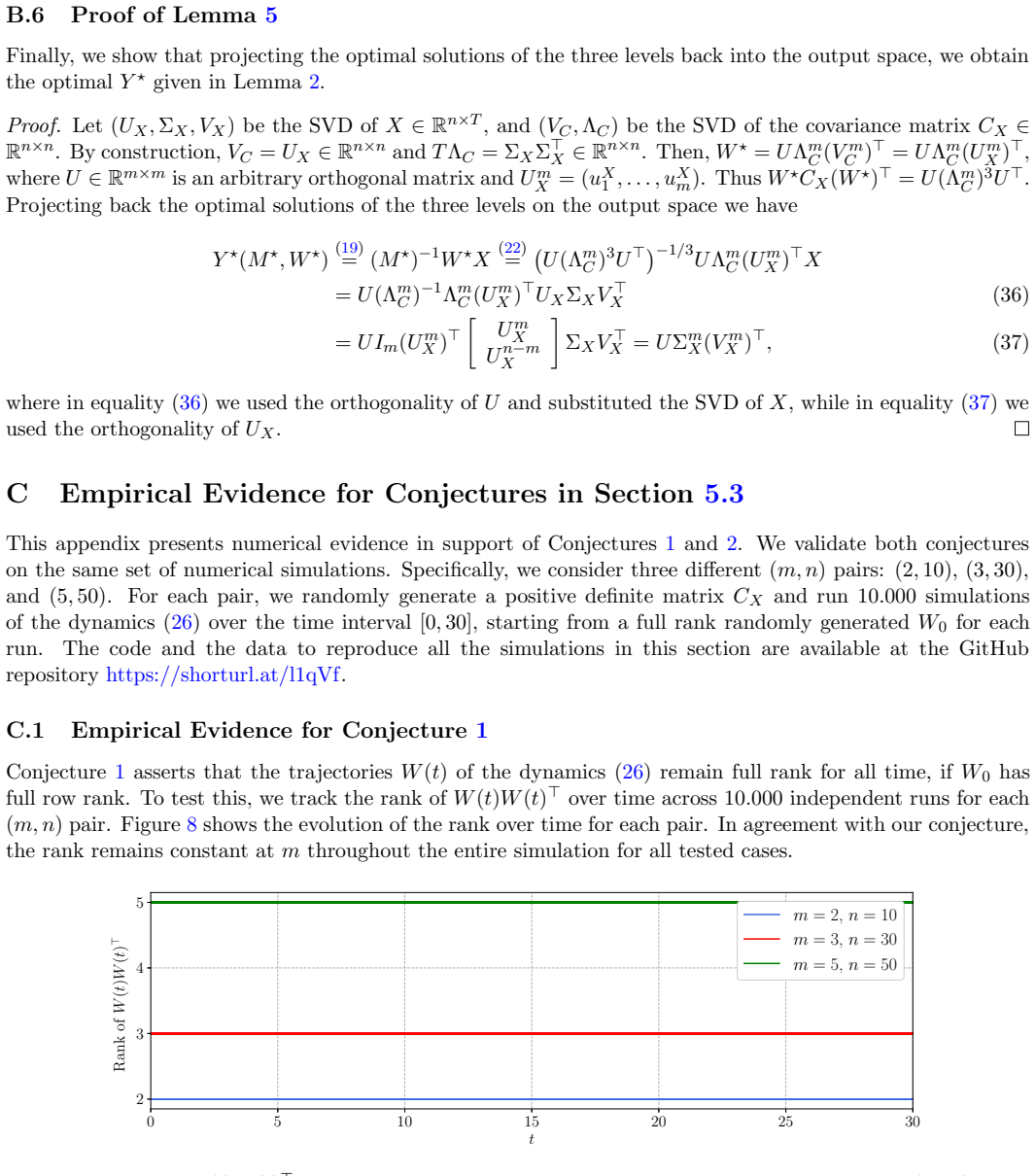
- ad hoc to paper The slow dynamics (26) is well posed because W(t) remains full row rank (Conjecture 1).
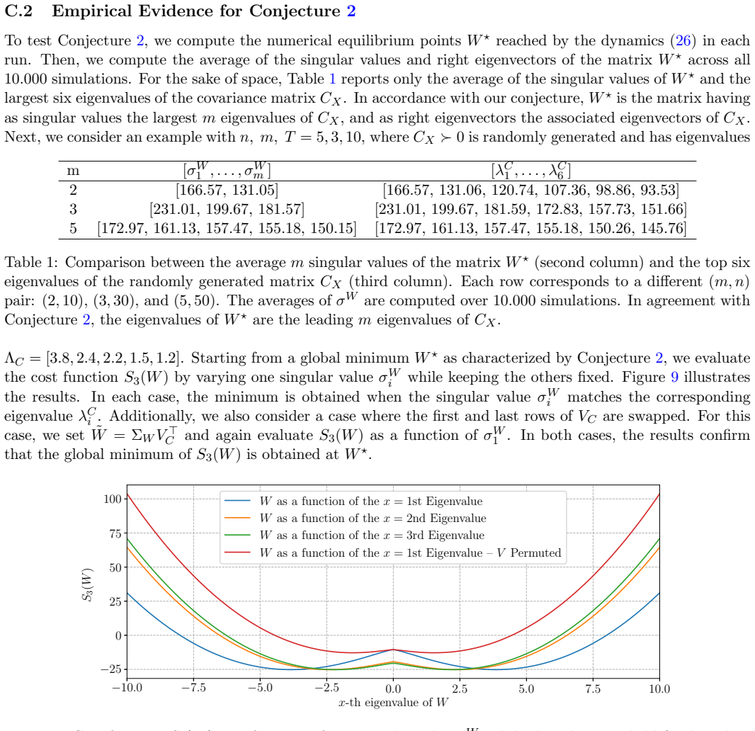
- ad hoc to paper Every non-global stationary point of S3 in the full-rank set is a strict saddle or maximum (Conjecture 2).
- ad hoc to paper If U^T Lambda1^T (Lambda1 U Lambda2 U^T Lambda1^T)^(-1/3) Lambda1 U is diagonal, then U is a permutation matrix (Conjecture 3).
- domain assumption Saddle point property for the min-max interchange in the embedding (5) from [37, Appendix A, Proposition 1].
- standard math Kachurovskii theorem (Lemma 1), LaSalle invariance, and the strict-saddle escape result of [12, Corollary 4].
Cite this review
Pith. "Pith review of Similarity Matching Networks: Hebbian Learning and Convergence Over Multiple Time Scales." pith.science (2026). https://pith.science/paper/UMGOMBZJ
@misc{pith2026250606134,
  author       = {Pith},
  title        = {Pith review of: Similarity Matching Networks: Hebbian Learning and Convergence Over Multiple Time Scales},
  year         = {2026},
  howpublished = {\url{https://pith.science/paper/UMGOMBZJ}},
  note         = {Machine review of arXiv:2506.06134}
}
read the original abstract
A recent breakthrough in biologically-plausible normative frameworks for dimensionality reduction is based upon the similarity matching cost function and the low-rank matrix approximation problem. Despite clear biological interpretation, successful application in several domains, and experimental validation, a formal complete convergence analysis remains elusive. Building on this framework, we consider and analyze a continuous-time neural network, the \emph{similarity matching network}, for principal subspace projection. Derived from a min-max-min objective, this biologically-plausible network consists of three coupled dynamics evolving at different time scales: neural dynamics, lateral synaptic dynamics, and feedforward synaptic dynamics at the fast, intermediate, and slow time scales, respectively. The feedforward and lateral synaptic dynamics consist of Hebbian and anti-Hebbian learning rules, respectively. By leveraging a multilevel optimization framework, we prove convergence of the dynamics in the offline setting. Specifically, at the first level (fast time scale), we show strong convexity of the cost function and global exponential convergence of the corresponding gradient-flow dynamics. At the second level (intermediate time scale), we prove strong concavity of the cost function and exponential convergence of the corresponding gradient-flow dynamics within the space of positive definite matrices. At the third and final level (slow time scale), we study a non-convex and non-smooth cost function, provide explicit expressions for its global minima, and prove almost sure convergence of the corresponding gradient-flow dynamics to the global minima. These results rely on two empirically motivated conjectures that are supported by thorough numerical experiments. Finally, we validate the effectiveness of our approach via a numerical example.
Figures


Figures from the paper (6 more)


Reference graph
Works this paper leans on
-
[1]
A. Balavoine, J. Romberg, and C. J. Rozell. Convergence and rate analysis of neural networks for sparse approximation.IEEE Transactions on Neural Networks and Learning Systems, 23(9):1377–1389, 2012. doi:10.1109/tnnls.2012.2202400
-
[2]
H. B. Barlow. Single units and sensation: a neuron doctrine for perceptual psychology?Perception, 1(4):371–394, 1972.doi:10.1068/p010371
-
[3]
Bullo.Contraction Theory for Dynamical Systems
F. Bullo.Contraction Theory for Dynamical Systems. Kindle Direct Publishing, 1.2 edition, 2024, ISBN 979-8836646806. URL: https://fbullo.github.io/ctds
work page 2024
-
[4]
V. Centorrino, F. Bullo, and G. Russo. Modelling and contractivity of neural-synaptic networks with Hebbian learning.Automatica, 164:111636, 2024.doi:10.1016/j.automatica.2024.111636
arXiv 2024
-
[5]
V. Centorrino, A. Gokhale, A. Davydov, G. Russo, and F. Bullo. Positive competitive networks for sparse reconstruction.Neural Computation, 36(6):1163–1197, 2024.doi:10.1162/neco_a_01657
-
[6]
L. Chang and D. Y. Tsao. The code for facial identity in the primate brain.Cell, 169(6):1013–1028.e14, June 2017.doi:10.1016/j.cell.2017.05.011
-
[7]
N. M. Chapochnikov, C. Pehlevan, and D. B. Chklovskii. Normative and mechanistic model of an adaptive circuit for efficient encoding and feature extraction.Proceedings of the National Academy of Sciences, 120(29), 2023.doi:10.1073/pnas.2117484120
-
[8]
M. M. Churchland, J. P. Cunningham, M. T. Kaufman, J. D. Foster, P. Nuyujukian, S. I. Ryu, and K. V. Shenoy. Neural population dynamics during reaching.Nature, 487(7405):51–56, 2012.doi:10.1038/ nature11129
work page 2012
Show all 42 references
-
[9]
D. G. Clark and L. F. Abbott. Theory of coupled neuronal-synaptic dynamics.Physical Review X, 14(2):021001, 2024.doi:10.1103/PhysRevX.14.021001
2024 doi
- [10]
-
[11]
T. F. Cox and M. A. Cox.Multidimensional Scaling. CRC Press, 2000
2000
-
[12]
A. C. B. de Oliveira, M. Siami, and E. D. Sontag. Convergence analysis of overparametrized LQR formu- lations.arXiv preprint arXiv:2408.15456, 2024. 26
2024 arXiv
-
[13]
D. W. Dong and J. J. Hopfield. Dynamic properties of neural networks with adapting synapses.Network: Computation in Neural Systems, 3(3):267–283, 1992.doi:10.1088/0954-898x_3_3_002
1992 doi
-
[14]
F¨ oldi´ ak
P. F¨ oldi´ ak. Forming sparse representations by local anti-Hebbian learning.Biological Cybernetics, 64(2):165–70, 1990.doi:10.1007/BF02331346
1990 doi
-
[15]
Galtier, O
M. Galtier, O. Faugeras, and P. Bressloff. Hebbian learning of recurrent connections: A geometrical perspective.Neural Computation, 24:2346–83, 05 2012.doi:10.1162/NECO_a_00322
2012 doi
-
[16]
Gerstner and W
W. Gerstner and W. Kistler. Mathematical formulations of Hebbian learning.Biological Cybernetics, 87:404–15, 2003.doi:10.1007/s00422-002-0353-y
2003 doi
-
[17]
Gerstner, W
W. Gerstner, W. M. Kistler, R. Naud, and L. Paninski.Neuronal Dynamics: From Single Neurons To Networks and Models of Cognition. Cambridge University Press, 2014, ISBN 9781107635197. URL: https: //neuronaldynamics.epfl.ch
2014
-
[18]
D. O. Hebb.The Organization of Behavior: A Neuropsychological Theory. John Wiley & Sons, 1949. doi:10.1002/sce.37303405110
1949 doi
-
[19]
M. W. Hirsch and S. Smale.Differential Equations, Dynamical Systems and Linear Algebra. Academic Press, 1974, ISBN 0123495504
1974
-
[20]
J. J. Hopfield and D. W. Tank. Computing with neural circuits: A model.Science, 233(4764):625–633, 1986.doi:10.1126/science.3755256
1986 doi
-
[21]
R. A. Horn and C. R. Johnson.Matrix Analysis. Cambridge University Press, 2nd edition, 2012, ISBN 0521548233
2012
-
[23]
D. H. Hubel and T. N. Wiesel. Receptive fields and functional architecture of monkey striate cortex.The Journal of Physiology, 195(1):215–243, 1968.doi:10.1113/jphysiol.1968.sp008455
1968 doi
-
[24]
R. I. Kachurovskii. Monotone operators and convex functionals.Uspekhi Matematicheskikh Nauk, 15(4):213–215, 1960
1960
-
[25]
Kozachkov, M
L. Kozachkov, M. Lundqvist, J.-J. E. Slotine, and E. K. Miller. Achieving stable dynamics in neural circuits.PLoS Computational Biology, 16(8):1–15, 2020.doi:10.1371/journal.pcbi.1007659
2020 doi
-
[26]
Lipshutz, C
D. Lipshutz, C. Pehlevan, and D. B. Chklovskii. Biologically plausible single-layer networks for nonnegative independent component analysis.Biological Cybernetics, 2022.doi:10.1007/s00422-022-00943-8
2022 doi
-
[27]
X. Liu, Z. Wen, and Y. Zhang. An efficient Gauss–Newton algorithm for symmetric low-rank product matrix approximations.SIAM Journal on Optimization, 25(3):1571–1608, 2015.doi:10.1137/140971464
2015 doi
-
[28]
Lohmiller and J.-J
W. Lohmiller and J.-J. E. Slotine. On contraction analysis for non-linear systems.Automatica, 34(6):683– 696, 1998.doi:10.1016/S0005-1098(98)00019-3
1998 doi
-
[29]
Lojasiewicz
S. Lojasiewicz. Sur les trajectoires du gradient d’une fonction analytique.Seminari di Geometria 1982- 1983, pages 115–117, 1984. Istituto di Geometria, Dipartimento di Matematica, Universit` a di Bologna, Italy
1982
-
[30]
E. Oja. Simplified neuron model as a principal component analyzer.Journal of Mathematical Biology, 15(3):267–273, 1982.doi:10.1007/bf00275687
1982 doi
-
[31]
B. A. Olshausen and D. J. Field. Emergence of simple-cell receptive field properties by learning a sparse code for natural images.Nature, 381(6583):607–609, 1996.doi:10.1038/381607a0. 27
1996 doi
-
[32]
Pehlevan and D
C. Pehlevan and D. Chklovskii. A normative theory of adaptive dimensionality reduction in neural networks. Advances in Neural Information Processing Systems, 28, 2015
2015
-
[33]
Pehlevan and D
C. Pehlevan and D. B. Chklovskii. A Hebbian/Anti-Hebbian network derived from online non-negative matrix factorization can cluster and discover sparse features. InAsilomar Conference on Signals, Systems and Computers, pages 769–775, 2014.doi:10.1109/ACSSC.2014.7094553
2014
-
[34]
Pehlevan and D
C. Pehlevan and D. B. Chklovskii. Neuroscience-inspired online unsupervised learning algorithms: Artificial neural networks.IEEE Signal Processing Magazine, 36(6):88–96, 2019.doi:10.1109/msp.2019.2933846
2019
-
[35]
Pehlevan, T
C. Pehlevan, T. Hu, and D. B. Chklovskii. A Hebbian/Anti-Hebbian neural network for linear subspace learning: A derivation from multidimensional scaling of streaming data.Neural Computation, 27(7):1461– 1495, 2015.doi:10.1162/neco_a_00745
2015 doi
-
[36]
Pehlevan, S
C. Pehlevan, S. Mohan, and D. B. Chklovskii. Blind nonnegative source separation using biological neural networks.Neural Computation, 29(11):2925–2954, 2017.doi:10.1162/neco_a_01007
2017 doi
-
[37]
Pehlevan, A
C. Pehlevan, A. M. Sengupta, and D. B. Chklovskii. Why do similarity matching objectives lead to Hebbian/anti-Hebbian networks?Neural Computation, 30(1):84–124, 2017.doi:10.1162/neco_a_01018
2017 doi
-
[38]
Russo, M
G. Russo, M. Di Bernardo, and E. D. Sontag. Global entrainment of transcriptional systems to periodic inputs.PLoS Computational Biology, 6(4):e1000739, 2010.doi:10.1371/journal.pcbi.1000739
2010 doi
-
[39]
Saxena and J
S. Saxena and J. P. Cunningham. Towards the neural population doctrine.Current Opinion in Neurobi- ology, 55:103–111, 2019.doi:10.1016/j.conb.2019.02.002
2019 doi
-
[40]
Scellier and Y
B. Scellier and Y. Bengio. Equilibrium propagation: Bridging the gap between energy-based models and backpropagation.Frontiers in Computational Neuroscience, 11:24, 2017.doi:10.3389/fncom.2017. 00024
2017 doi
-
[41]
P. M. Wensing and J.-J. E. Slotine. Beyond convexity — Contraction and global convergence of gradient descent.PLoS One, 15(8):1–29, 2020.doi:10.1371/journal.pone.0236661
2020 doi
-
[42]
Wright and Y
J. Wright and Y. Ma.High-Dimensional Data Analysis with Low-Dimensional Models: Principles, Com- putation, and Applications. Cambridge University Press, 2022
2022
-
[43]
S. Xie, G. Russo, and R. H. Middleton. Scalability in nonlinear network systems affected by delays and disturbances.IEEE Transactions on Control of Network Systems, 8(3):1128–1138, 2021.doi:10.1109/ TCNS.2021.3058934. 28
2021
Reviewed August 7, 2026 · model on record in the stance chip above.
Discussion (0). Sign in to comment.