Statistical Machine Learning for Astronomy -- A Textbook

Yuan-Sen Ting

REVIEW 2 major objections 5 minor 1 cited by

Statistical Machine Learning for Astronomy -- A Textbook

T0 review · 2 major / 5 minor · reviewed 2026-08-07 · deepseek-v4-flash

Challenge this review Re-run · record.json Download PDF Read on arXiv ↗

Pith's one-line read A new astronomy textbook argues that machine learning, from linear regression to neural networks, is a continuation of Bayesian inference.

desk verdict A serious, well-written theory-first textbook for astronomy ML, with an 'everything is Bayesian' framing that is asserted more than proved; worth a proper referee. read the letter →

arxiv 2506.12230 v1 pith:W4CP3DMR submitted 2025-06-13 astro-ph.IM cs.LGstat.APstat.ML

Yuan-Sen Ting This is my paper

classification astro-ph.IMcs.LGstat.APstat.ML MSC 62F1562J0568T05

keywords astronomymachinelearningBayesianinferenceuncertaintyquantificationneuralnetworksGaussianprocessestextbook

verification ladder T0 review T1 audit T2 compute T3 formal

The pith

A machine-rendered reading of the paper's core claim, the machinery that carries it, and where it could break.

The reading

This textbook tries to establish a specific way of understanding machine learning: rather than a toolbox of black boxes, ML is a continuation of the statistical methods astronomers already use, all emerging from the same probability theory and Bayesian inference. The intended payoff is pedagogical and practical: if a reader masters Bayes' theorem and the idea of treating parameters as random variables, they can derive linear regression, classification, PCA, clustering, Gaussian processes, and even neural networks as successive instances of one inference framework. That matters for astronomy because large surveys now make automated analysis unavoidable, and the field is split between enthusiastic adoption and suspicion of 'black box' methods. The book's claim is that this split rests on a misunderstanding, and that uncertainty quantification, the core of scientific inference, can be preserved through the whole hierarchy of methods.

What carries the argument

The load-bearing object is Bayes' theorem in its proportional form, $p(\theta|D) \propto p(D|\theta)p(\theta)$, used as an organizing derivation chain that treats both data and model parameters as random variables. Each chapter obtains a standard machine learning algorithm by making specific choices inside this framework: Gaussian likelihoods give linear regression, conjugate priors give Bayesian linear regression, a Laplace approximation gives Bayesian logistic regression, constrained optimization gives PCA, expectation-maximization on hidden variables gives K-means and Gaussian mixture models, detailed balance gives Metropolis-Hastings and Gibbs samplers, and the kernel trick turns Bayesian linear regression into Gaussian processes. The book also leans on the 'modeling-learning spectrum' and the concept of inductive bias as conceptual glue for relating physical modeling to data-driven learning.

What would settle it

Take a standard neural network trained by stochastic gradient descent on a cross-entropy loss, and ask whether any Bayesian posterior over weights, under any reasonable prior and likelihood, produces the same predictive distribution; if even one standard training setup cannot be matched by a coherent posterior, the central claim that neural networks are natural extensions of Bayesian inference fails as a mathematical statement rather than a metaphor.

Watch

Extended reading notes

Core claim

The textbook's central claim is that machine learning is not a separate discipline from classical statistics but a continuation of it: every method treated, from linear regression and logistic regression through PCA, K-means, Gaussian mixture models, MCMC sampling, and Gaussian processes up to neural networks, can be derived from the same probability theory and Bayesian inference principles that underlie all scientific data analysis. By treating model parameters as random variables and updating beliefs through Bayes' theorem, each technique becomes an instance of one inference machinery, differing only in complexity, tractability, and inductive bias. The book presents itself not as a new research contribution but as a pedagogical synthesis, systematically deriving established methods from first principles so that readers can understand why algorithms work, when they are appropriate, and how they connect to broader statistical principles.

Load-bearing premise

The load-bearing premise is that neural network training is genuinely a form of Bayesian inference, rather than an optimization procedure that merely looks like one, and the book asserts this organizing principle without proving a formal equivalence.

Editorial extensions

If this is right

A reader who follows the textbook's sequence should be able to derive seemingly unrelated algorithms from one probabilistic framework, reducing the need to treat each method as an isolated recipe.
Uncertainty quantification becomes the default concern at every level of the hierarchy, so adopting machine learning methods need not mean abandoning the error bars and rigor that astronomy requires.
Neural networks are repositioned as the flexible end of a continuous spectrum rather than a break with statistics, which could ease the polarization between enthusiasts and skeptics in the field.
Classical methods with analytical solutions, such as linear regression and PCA, become testbeds for validating the behavior of more complex methods before applying them to scientific questions.
The textbook's structure offers a ready-made curriculum for graduate courses that want to teach modern machine learning from its statistical foundations rather than as an engineering subject.

Reading between the lines

Editorial extensions of the paper, not claims the author makes directly.

If the book's unification is taken literally, it suggests a concrete research program: recast stochastic gradient descent as an approximate Bayesian inference procedure, for instance through a stochastic-gradient Langevin or variational treatment, and test whether the resulting uncertainty is calibrated on benchmark astronomical datasets.
The book's case against the 'black box' label depends on practical uncertainty approximations, such as Monte Carlo dropout, being well calibrated; that is an empirical question the text leaves open.
The same organizing principle could be extended to simulation-based inference and foundation models, which the book mentions but does not fully integrate into its classical-to-modern derivation chain.
A curriculum experiment could test the pedagogical claim directly: teach one group with this derivation-first Bayesian sequence and another with an algorithm-first approach, then measure how well each group transfers to unfamiliar machine learning methods.

Share X Bluesky LinkedIn Reddit HN

Editorial analysis

A structured set of objections, weighed in public.

Desk editor's note, referee report, and a circularity audit.

Desk Editor's Note

read the letter

Quick take: this is a real textbook, not a research preprint, and it knows it. The author explicitly disclaims new theoretical results and instead tries to give astronomy grad students a theory-first, Bayesian-flavored path from probability to neural networks. If you teach ML for astronomers, it's worth a look; if you're scanning for new science, there is none, and that's fine.

The sampled chapters are mathematically careful. Chapters 2-4 derivations are correct: law of total expectation, variance algebra, the one-data-point Bayesian updating examples, and the MLE-to-Bayesian regression progression all check out. The figures are well designed, and the astronomical examples (Kepler, M-sigma, Kennicutt-Schmidt) are genuinely integrated into the math, not decorative. The book also ships a GitHub repo with tutorials, which is real support for a textbook. As a synthesis, it fills a genuine gap: most astro ML books are application-heavy; this one insists on deriving things from first principles.

The soft spot is the central thesis. The preface promises that all ML techniques 'emerge from the same probability theory and Bayesian inference principles,' and Chapter 2 says each technique 'implements the core Bayesian idea of updating our beliefs about model parameters based on observed data.' The derivations don't actually deliver that. MLE is point estimation; PCA is constrained variance maximization; k-means is EM maximizing likelihood; neural networks are loss minimization with SGD. The book does have genuinely Bayesian chapters, but they are separate, and the preface itself admits neural networks involve a 'departure from fully Bayesian approaches.' So the unifying claim is an interpretive lens, not a theorem derived in the text. That is a real soft spot, but not fatal: a textbook is allowed to have a point of view. It just should be framed as a perspective, not as something the math proves, because a student who absorbs the framing uncritically could mistake point-estimate tools for full posterior inference.

I also could not verify the later chapters (sampling, MCMC, Gaussian processes, neural networks) from the available material; the sampled chapters are solid, but the rest needs checking.

Who this is for: astronomy grad students and researchers who want the mathematical underbelly of ML before applying it. It deserves a serious referee. Have a referee read the framing chapter plus chapters 10, 11, and 15 to check whether the 'Bayesian everything' claim holds up. If the later chapters are as careful as the early ones, this is a useful textbook with an overstated but harmless thesis. My recommendation: engage.

Referee Report

2 major / 5 minor

Summary. The manuscript is a draft textbook rather than a research paper. It proposes a unified presentation of statistical machine learning for astronomy built around Bayesian inference, with the explicit thesis that machine learning techniques are natural extensions of the probability theory and Bayesian principles used in classical astronomical data analysis. The reviewed portion contains the Preface/Overview, full chapters on Bayesian inference and summary statistics, and the opening of the linear regression chapter. The text is expository: it derives moments, expectation, variance, covariance, the laws of total expectation and total variance, bootstrap resampling, and the first steps of maximum-likelihood linear regression, with astronomical examples and Further Reading sections.

Significance. The available chapters are generally sound and clearly written. The derivations I checked—law of total expectation (§3.4), law of total variance (§3.8), variance and covariance algebra (§3.5, §3.6), and the correlation bound via the Cauchy-Schwarz inequality (§3.5)—are correct, and the worked example of Bayesian updating with a single roll of a die (§2.7.1) is a helpful pedagogical device. The emphasis on assumptions and limitations, such as the discussion of bootstrap limitations in §3.7 and the treatment of inductive bias in Chapter 1, is a genuine strength. However, the overarching claim that all discussed machine learning methods, including PCA, k-means, and neural networks, emerge from Bayesian inference is not demonstrated in the reviewed text and is in tension with the book's own statement that neural networks represent a departure from fully Bayesian approaches. The significance of the book therefore depends on whether the later chapters close this gap.

major comments (2)

[§1 (pp. 11–16), §2 (p. 22), §4.3] The central organizing claim—that every method in the book 'implements the core Bayesian idea of updating our beliefs about model parameters based on observed data'—is asserted but not supported by the derivations in the available text. Maximum likelihood in §4.3 is derived as a point-estimation procedure, and the Preface itself states that neural networks involve a 'departure from fully Bayesian approaches' (p. 16). No derivation in the reviewed chapters shows that PCA (§10.4), k-means (§11.2), or standard neural-network training (§15.3) is a form of posterior inference. Because the book's pedagogical value proposition rests on the coherence of the Bayesian framework, the Preface and Chapter 2 should either qualify the claim to the sense in which these methods can be viewed within a common probabilistic framework, or add a systematic treatment that states exactly when each method admits a Bayesian decision-theoretic or MAP interpretation and where the equivalence fails.
[Table 2.1 (§2.7.1)] The columns for the 'Worse' and 'Worst' die models do not sum to 1: they sum to 25/24 and 41/40, respectively. This contradicts the sentence in §2.7.1 that 'for each model θ, the probabilities p(D|θ) must sum to one—this is reflected in how each column in our table sums to unity.' The subsequent posterior calculations are internally correct because they normalize the row likelihoods, but the table and the accompanying claim must be corrected; this worked example is the book's primary demonstration of Bayesian updating, and a normalization error is especially misleading here.

minor comments (5)

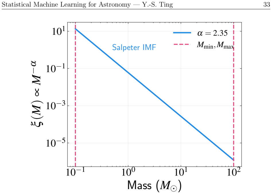
[§2.3, Eq. (2.10)] The normalized power-law formula is valid only for α ≠ 1; the logarithmic normalizing case for α = 1 should be noted for completeness.
[§3.2, Eq. (3.7)] The linear transformation formula for probability densities should state explicitly that it assumes a ≠ 0.
[Further Reading sections] The text cites works such as Efron [1979] and Gelman et al. [2013], but no reference list appears in the reviewed excerpt; the final manuscript should include complete bibliographic entries.
[General] Several displayed equations in the provided text appear with broken spacing and odd characters, for example Eq. (2.5) and Eq. (3.77); the compiled version should be checked for correct rendering.
[Chapter 4 heading] The chapter heading reads 'Chapter 4: Linear Regression' while the table of contents uses '4 Linear Regression'; the duplicated numbering and title should be made consistent.

Circularity Check

0 steps flagged · score 0.0 of 10

Textbook is an explicit pedagogical synthesis of established results; no circular derivation chain found.

full rationale

This is a textbook, not a claim of new theoretical results. Chapter 1 states explicitly: 'It is important to emphasize that this textbook does not claim to present new theoretical results or novel algorithmic developments... Our role is thus one of curation and pedagogical organization rather than original research—collecting, connecting, and presenting established results in a way that builds systematic understanding for astronomical researchers.' Because the book disclaims originality and does not derive new predictions from fitted parameters, the standard circularity patterns (self-definitional equations, fitted inputs renamed as predictions, self-citation chains, or imported uniqueness theorems) do not apply. The central organizing thesis—that machine learning techniques 'emerge from the same probability theory and Bayesian inference principles'—is presented as an interpretive and pedagogical lens, not as a theorem derived from those principles. The book itself qualifies the claim for neural networks: they 'appear not as a departure from previous methods but as a natural extension that trades some of the mathematical tractability and uncertainty quantification of classical methods for greater computational scalability and flexibility,' and the Preface mentions the 'departure from fully Bayesian approaches' for standard network training. Thus the framework assertion is deliberately hedged rather than asserted as a full equivalence. Individual chapters derive standard results from their own stated assumptions (e.g., MLE in Chapter 4 from likelihood principles, PCA in Section 10.4 via Lagrange multipliers, EM for K-means/GMMs in Chapter 11), and the reference lists point to external classical sources such as Fisher, Jaynes, and Gelman rather than to the author's own prior work as the load-bearing justification. No equation in the supplied text reduces to its own input, and no parameter fitted to a subset is later reported as an independent prediction. The strongest concern raised by a skeptical reader—that the unifying Bayesian claim is asserted rather than exhaustively demonstrated for optimization-based methods—is a scope or framing issue, not a circularity in the derivation chain. Under the review rules, an unsupported or non-standard framing should be recorded as a correctness or pedagogy concern, not as circularity. Therefore the circularity score is 0.

Assumptions & free parameters 0 free parameters · 4 assumptions · 0 invented entities

No free parameters are fitted and no new entities are introduced. The book relies on standard probability theory and the Bayesian interpretation as an organizing principle.

assumptions (4)

standard math Kolmogorov probability axioms (non-negativity, normalization, additivity)
Invoked in Chapter 2.2 as the basis of probability theory.
standard math Central Limit Theorem
Invoked in Chapter 2.3 to justify the ubiquity of Gaussian distributions for additive measurement noise.
domain assumption Treating model parameters as random variables
The book's core Bayesian interpretation, introduced in Chapter 2; it is a philosophical choice, not a theorem, and it underpins the entire framework.
domain assumption Astronomical measurements have heteroscedastic uncertainties that must be modeled
Motivates Chapter 6 on regression with input uncertainties, stated in the Preface as a unique challenge of astronomy.

how reviews work

0 comments

Cite this review

Pith. "Pith review of Statistical Machine Learning for Astronomy -- A Textbook." pith.science (2026). https://pith.science/paper/W4CP3DMR

@misc{pith2026250612230,
  author       = {Pith},
  title        = {Pith review of: Statistical Machine Learning for Astronomy -- A Textbook},
  year         = {2026},
  howpublished = {\url{https://pith.science/paper/W4CP3DMR}},
  note         = {Machine review of arXiv:2506.12230}
}

read the original abstract

This textbook provides a systematic treatment of statistical machine learning for astronomical research through the lens of Bayesian inference, developing a unified framework that reveals connections between modern data analysis techniques and traditional statistical methods. We show how these techniques emerge from familiar statistical foundations. The consistently Bayesian perspective prioritizes uncertainty quantification and statistical rigor essential for scientific inference in astronomy. The textbook progresses from probability theory and Bayesian inference through supervised learning including linear regression with measurement uncertainties, logistic regression, and classification. Unsupervised learning topics cover Principal Component Analysis and clustering methods. We then introduce computational techniques through sampling and Markov Chain Monte Carlo, followed by Gaussian Processes as probabilistic nonparametric methods and neural networks within the broader statistical context. Our theory-focused pedagogical approach derives each method from first principles with complete mathematical development, emphasizing statistical insight and complementing with astronomical applications. We prioritize understanding why algorithms work, when they are appropriate, and how they connect to broader statistical principles. The treatment builds toward modern techniques including neural networks through a solid foundation in classical methods and their theoretical underpinnings. This foundation enables thoughtful application of these methods to astronomical research, ensuring proper consideration of assumptions, limitations, and uncertainty propagation essential for advancing astronomical knowledge in the era of large astronomical surveys.

Figures

Figures reproduced from arXiv: 2506.12230 by the authors.

**Figure 2.1.** Illustration of deterministic versus random variables. The dashed vertical line [PITH_FULL_IMAGE:figures/full_fig_p024_2_1.png] view at source ↗

**Figure 2.2.** Visualization of a standard normal (Gaussian) distribution with mean [PITH_FULL_IMAGE:figures/full_fig_p029_2_2.png] view at source ↗

**Figure 2.3.** Visualization of a Poisson distribution with mean rate parameter [PITH_FULL_IMAGE:figures/full_fig_p031_2_3.png] view at source ↗

Figures from the paper (148 more)

**Figure 2.4.** Figure 2.4: Illustration of how the Poisson distribution (blue bars) approaches a Gaussian [PITH_FULL_IMAGE:figures/full_fig_p032_2_4.png]

**Figure 2.5.** Figure 2.5: Visualization of a power law distribution using the Salpeter Initial Mass Func [PITH_FULL_IMAGE:figures/full_fig_p033_2_5.png]

**Figure 2.6.** Figure 2.6: Illustration of joint and conditional probability distributions using stellar temper [PITH_FULL_IMAGE:figures/full_fig_p036_2_6.png]

**Figure 2.7.** Figure 2.7: Visualization of marginalization for a bivariate Gaussian distribution. The cen [PITH_FULL_IMAGE:figures/full_fig_p038_2_7.png]

**Figure 2.8.** Figure 2.8: Visualization of dependent versus independent variables. Left panels show a case [PITH_FULL_IMAGE:figures/full_fig_p041_2_8.png]

**Figure 2.9.** Figure 2.9: Top panel: Likelihood functions p(x|µ) for different proposed values of µ. When µ = 2 (red curve), the probability of measuring x = 6 is very low. When µ = 5 (green curve), this probability is much higher. Bottom panel: The likelihood p({6}|µ) as a function of µ, sho…

**Figure 2.10.** Figure 2.10: Top panel: Individual likelihood functions for different values of [PITH_FULL_IMAGE:figures/full_fig_p052_2_10.png]

**Figure 3.1.** Figure 3.1: Visualization of how different moments weight a probability distribution. Top [PITH_FULL_IMAGE:figures/full_fig_p060_3_1.png]

**Figure 3.2.** Figure 3.2: Visualization of how probability distributions transform under linear transfor [PITH_FULL_IMAGE:figures/full_fig_p063_3_2.png]

**Figure 3.3.** Figure 3.3: Visualization of expectation’s linearity property using a bivariate Gaussian dis [PITH_FULL_IMAGE:figures/full_fig_p068_3_3.png]

**Figure 3.4.** Figure 3.4: Visualization of expectation’s additivity property using bivariate Gaussian dis [PITH_FULL_IMAGE:figures/full_fig_p069_3_4.png]

**Figure 3.5.** Figure 3.5: Visualization of the law of total expectation using stellar mass-luminosity rela [PITH_FULL_IMAGE:figures/full_fig_p072_3_5.png]

**Figure 3.6.** Figure 3.6: Visualization of how variance and standard deviation transform under linear [PITH_FULL_IMAGE:figures/full_fig_p076_3_6.png]

**Figure 3.7.** Figure 3.7: Visualization of how correlation shapes bivariate normal distributions. The [PITH_FULL_IMAGE:figures/full_fig_p079_3_7.png]

**Figure 3.8.** Figure 3.8: Visualization of how variances add for independent random variables. Left [PITH_FULL_IMAGE:figures/full_fig_p083_3_8.png]

**Figure 3.9.** Figure 3.9: Demonstration of how sample mean uncertainty decreases with sample size. Left [PITH_FULL_IMAGE:figures/full_fig_p085_3_9.png]

**Figure 3.10.** Figure 3.10: Illustration of the bootstrap resampling process and its ability to estimate [PITH_FULL_IMAGE:figures/full_fig_p088_3_10.png]

**Figure 3.11.** Figure 3.11: Visualization of the law of total variance using the stellar mass-luminosity [PITH_FULL_IMAGE:figures/full_fig_p092_3_11.png]

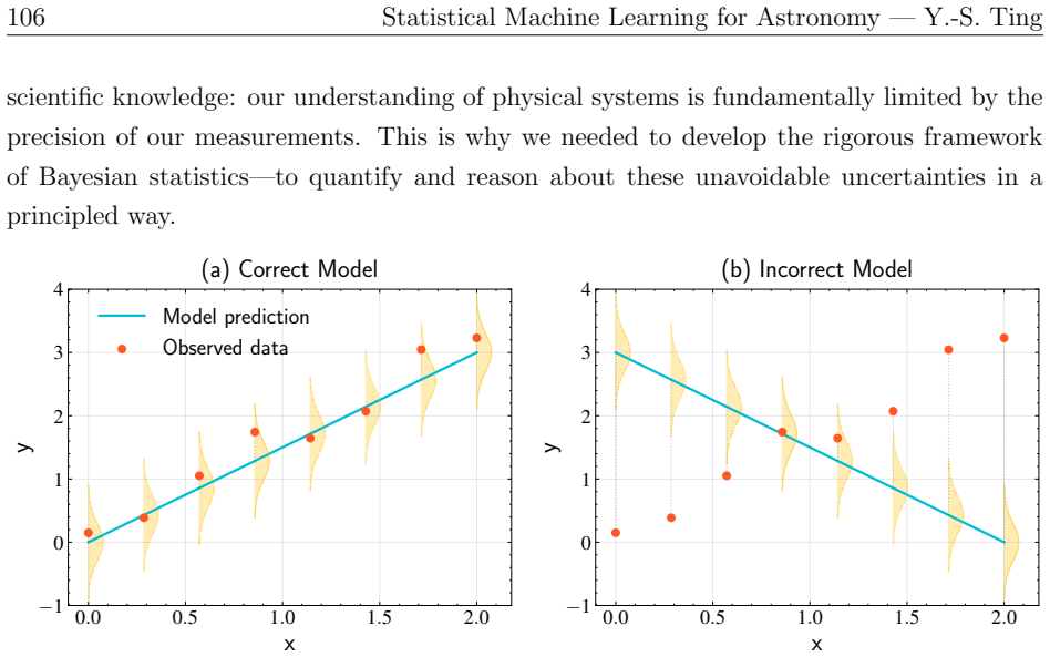
**Figure 4.1.** Figure 4.1: Visualization of the likelihood function for linear regression with Gaussian noise. [PITH_FULL_IMAGE:figures/full_fig_p106_4_1.png]

**Figure 4.2.** Figure 4.2: Demonstration of how different choices of uncertainty values affect the likelihood [PITH_FULL_IMAGE:figures/full_fig_p114_4_2.png]

**Figure 4.3.** Figure 4.3: Schematic illustration showing the globally convex log-likelihood surface in ( [PITH_FULL_IMAGE:figures/full_fig_p116_4_3.png]

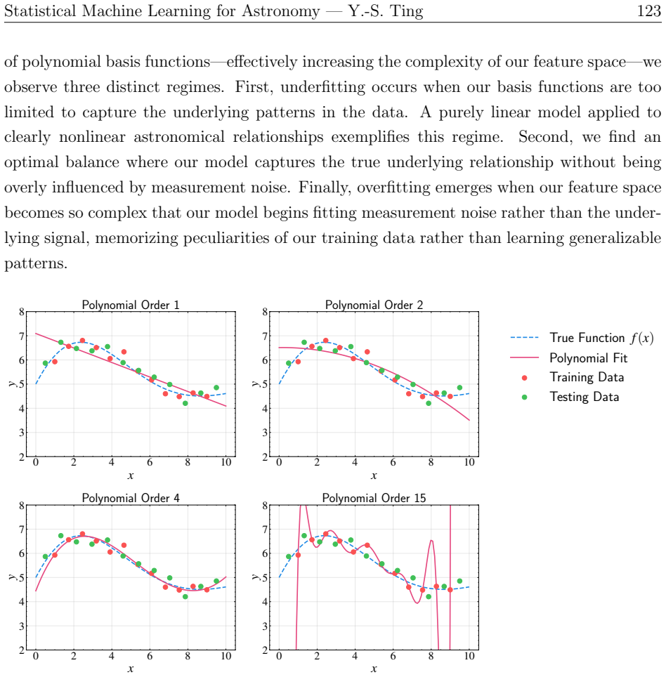
**Figure 4.4.** Figure 4.4: Demonstration of polynomial fitting with increasing model complexity. Each [PITH_FULL_IMAGE:figures/full_fig_p123_4_4.png]

**Figure 4.5.** Figure 4.5: Training and test error curves (on log scale) illustrating the three fundamental [PITH_FULL_IMAGE:figures/full_fig_p125_4_5.png]

**Figure 5.1.** Figure 5.1: Illustration of why we need to go beyond simple maximum likelihood estimation. [PITH_FULL_IMAGE:figures/full_fig_p130_5_1.png]

**Figure 5.2.** Figure 5.2: Visualization of Poisson-Gamma conjugacy in star count analysis. Panel (a) [PITH_FULL_IMAGE:figures/full_fig_p135_5_2.png]

**Figure 5.3.** Figure 5.3: Visualization of Gaussian conjugacy. Panel (a) demonstrates how multiplying [PITH_FULL_IMAGE:figures/full_fig_p140_5_3.png]

**Figure 5.4.** Figure 5.4: Visualization of the product of two 2D Gaussian distributions. The blue and [PITH_FULL_IMAGE:figures/full_fig_p143_5_4.png]

**Figure 5.5.** Figure 5.5: Comparison of maximum likelihood and Bayesian approaches to linear regression. [PITH_FULL_IMAGE:figures/full_fig_p145_5_5.png]

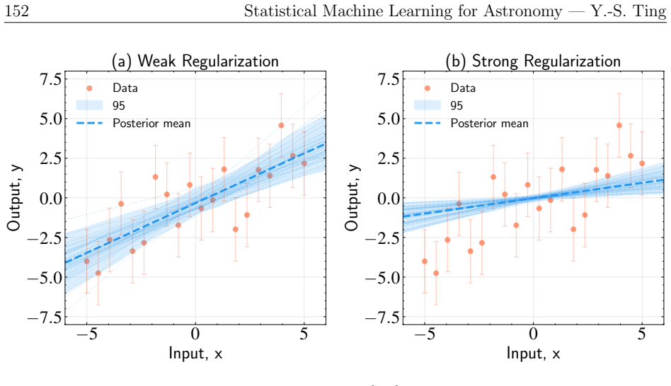
**Figure 5.6.** Figure 5.6: Effect of regularization strength (λ = σ 2/η2 ) in Bayesian linear regression. Panel (a) shows weak regularization (small λ, corresponding to precise measurements or uncertain prior), where the model has more freedom to fit the data, resulting in wider prediction ba…

**Figure 5.7.** Figure 5.7: Visualization of the posterior predictive distribution in Bayesian linear regression. [PITH_FULL_IMAGE:figures/full_fig_p154_5_7.png]

**Figure 6.1.** Figure 6.1: Illustration of how measurement uncertainties affect regression. Both panels [PITH_FULL_IMAGE:figures/full_fig_p166_6_1.png]

**Figure 6.2.** Figure 6.2: Demonstration of how measurement uncertainties affect the apparent dynamic [PITH_FULL_IMAGE:figures/full_fig_p168_6_2.png]

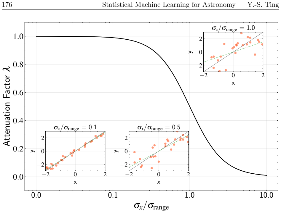
**Figure 6.3.** Figure 6.3: Demonstration of attenuation bias in parameter estimation. Both panels show [PITH_FULL_IMAGE:figures/full_fig_p174_6_3.png]

**Figure 6.4.** Figure 6.4: Demonstration of how measurement uncertainties affect parameter estimation [PITH_FULL_IMAGE:figures/full_fig_p176_6_4.png]

**Figure 6.5.** Figure 6.5: Demonstration of how we estimate true positions in a hierarchical model. Both [PITH_FULL_IMAGE:figures/full_fig_p181_6_5.png]

**Figure 6.6.** Figure 6.6: Demonstration of how Deming regression corrects for attenuation bias compared [PITH_FULL_IMAGE:figures/full_fig_p187_6_6.png]

**Figure 6.7.** Figure 6.7: Demonstration of heteroscedastic Deming regression and its numerical solu [PITH_FULL_IMAGE:figures/full_fig_p192_6_7.png]

**Figure 7.1.** Figure 7.1: Demonstration of binary classification in a two-dimensional feature space. Stars [PITH_FULL_IMAGE:figures/full_fig_p196_7_1.png]

**Figure 7.2.** Figure 7.2: Visualization of generative versus discriminative approaches in classification. [PITH_FULL_IMAGE:figures/full_fig_p199_7_2.png]

**Figure 7.3.** Figure 7.3: Illustration of the problem of simply treating classification as regression. Panel [PITH_FULL_IMAGE:figures/full_fig_p202_7_3.png]

**Figure 7.4.** Figure 7.4: Illustration of how direct linear regression can lead to suboptimal decision bound [PITH_FULL_IMAGE:figures/full_fig_p203_7_4.png]

**Figure 7.5.** Figure 7.5: The sigmoid function and its role in logistic regression. Panel (a) shows the [PITH_FULL_IMAGE:figures/full_fig_p204_7_5.png]

**Figure 7.6.** Figure 7.6: Visualization of how logistic regression transforms unbounded linear predictions [PITH_FULL_IMAGE:figures/full_fig_p205_7_6.png]

**Figure 7.7.** Figure 7.7: Illustration of how Gaussian generative models with equal covariance matrices [PITH_FULL_IMAGE:figures/full_fig_p207_7_7.png]

**Figure 7.8.** Figure 7.8: Illustration of how the covariance structure affects the optimal decision bound [PITH_FULL_IMAGE:figures/full_fig_p209_7_8.png]

**Figure 7.9.** Figure 7.9: Demonstration of how class priors affect the decision boundary in logistic re [PITH_FULL_IMAGE:figures/full_fig_p210_7_9.png]

**Figure 7.10.** Figure 7.10: Demonstration of how feature transformations can improve classification perfor [PITH_FULL_IMAGE:figures/full_fig_p213_7_10.png]

**Figure 7.11.** Figure 7.11: Visualization of gradient descent optimization in weight space. The contours [PITH_FULL_IMAGE:figures/full_fig_p219_7_11.png]

**Figure 7.12.** Figure 7.12: Visualization of gradient contributions in logistic regression. The plot shows [PITH_FULL_IMAGE:figures/full_fig_p222_7_12.png]

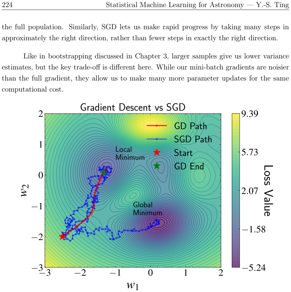
**Figure 7.13.** Figure 7.13: Comparison of Gradient Descent (GD) and Stochastic Gradient Descent tra [PITH_FULL_IMAGE:figures/full_fig_p224_7_13.png]

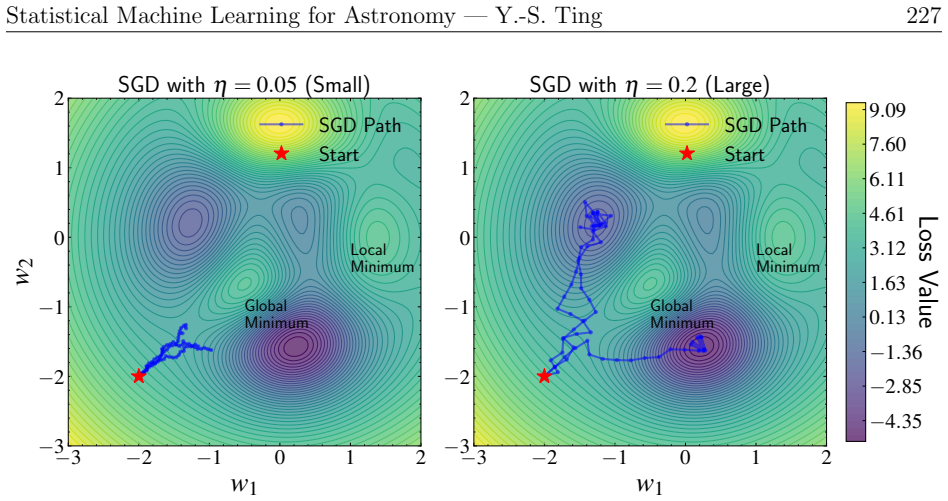
**Figure 7.14.** Figure 7.14: Comparison of Stochastic Gradient Descent behavior with different learning [PITH_FULL_IMAGE:figures/full_fig_p227_7_14.png]

**Figure 7.15.** Figure 7.15: Comparison of two learning rate scheduling strategies. [PITH_FULL_IMAGE:figures/full_fig_p228_7_15.png]

**Figure 8.1.** Figure 8.1: Illustration of pathological cases in One-vs-Rest (OvR) multi-class classification. [PITH_FULL_IMAGE:figures/full_fig_p237_8_1.png]

**Figure 8.2.** Figure 8.2: Illustration of the circular contradiction problem in One-vs-One classification [PITH_FULL_IMAGE:figures/full_fig_p238_8_2.png]

**Figure 8.3.** Figure 8.3: Visualization of how softmax-based multi-class classification ensures consistent [PITH_FULL_IMAGE:figures/full_fig_p248_8_3.png]

**Figure 8.4.** Figure 8.4: Extension of the softmax visualization to four classes, demonstrating how the [PITH_FULL_IMAGE:figures/full_fig_p249_8_4.png]

**Figure 8.5.** Figure 8.5: Comparison of (Pearson) correlation and mutual information for detecting sta [PITH_FULL_IMAGE:figures/full_fig_p254_8_5.png]

**Figure 9.1.** Figure 9.1: Comparison between standard and Bayesian approaches to logistic regression. [PITH_FULL_IMAGE:figures/full_fig_p274_9_1.png]

**Figure 9.2.** Figure 9.2: Visualization of the Laplace approximation principle. The true posterior distri [PITH_FULL_IMAGE:figures/full_fig_p279_9_2.png]

**Figure 9.3.** Figure 9.3: Visualization of the Bernstein-von Mises theorem, demonstrating why Laplace [PITH_FULL_IMAGE:figures/full_fig_p281_9_3.png]

**Figure 9.4.** Figure 9.4: Illustration of how boundary points affect uncertainty in Bayesian logistic regres [PITH_FULL_IMAGE:figures/full_fig_p290_9_4.png]

**Figure 9.5.** Figure 9.5: Bayesian logistic regression illustrated through multiple decision boundaries [PITH_FULL_IMAGE:figures/full_fig_p292_9_5.png]

**Figure 9.6.** Figure 9.6: Visualization of the dimensionality reduction from weight space to logit space [PITH_FULL_IMAGE:figures/full_fig_p294_9_6.png]

**Figure 9.7.** Figure 9.7: The probit function as the cumulative distribution function (CDF) of the stan [PITH_FULL_IMAGE:figures/full_fig_p296_9_7.png]

**Figure 9.8.** Figure 9.8: Comparison of the sigmoid function σ(x) with different scaled probit functions Φ(λx). The optimal scaling factor λ = p π/8 ≈ 0.63 (red dashed line) provides the best overall approximation to the sigmoid function (blue solid line). This scaling factor is derived by ma…

**Figure 9.9.** Figure 9.9: Comparison of standard and Bayesian logistic regression predictions. [PITH_FULL_IMAGE:figures/full_fig_p303_9_9.png]

**Figure 10.1.** Figure 10.1: Vector projection in 2D space, illustrating a key mathematical concept for PCA. [PITH_FULL_IMAGE:figures/full_fig_p313_10_1.png]

**Figure 10.2.** Figure 10.2: Visualization of Principal Component Analysis (PCA) for dimension reduction. [PITH_FULL_IMAGE:figures/full_fig_p315_10_2.png]

**Figure 10.3.** Figure 10.3: Geometric intuition of Lagrange multipliers. The contour lines represent the [PITH_FULL_IMAGE:figures/full_fig_p320_10_3.png]

**Figure 10.4.** Figure 10.4: Perpendicularity of the constraint gradient. This figure illustrates why the gra [PITH_FULL_IMAGE:figures/full_fig_p321_10_4.png]

**Figure 10.5.** Figure 10.5: Geometric visualization of how eigenvectors maintain their direction under [PITH_FULL_IMAGE:figures/full_fig_p326_10_5.png]

**Figure 10.6.** Figure 10.6: Visualization of how PCA identifies principal components using the covariance [PITH_FULL_IMAGE:figures/full_fig_p327_10_6.png]

**Figure 10.7.** Figure 10.7: Visualization of residual data after extracting the first principal component. [PITH_FULL_IMAGE:figures/full_fig_p332_10_7.png]

**Figure 10.8.** Figure 10.8: Scree plot for selecting the optimal number of principal components. The blue [PITH_FULL_IMAGE:figures/full_fig_p336_10_8.png]

**Figure 10.9.** Figure 10.9: Illustration of PCA’s limitation with multimodal data. [PITH_FULL_IMAGE:figures/full_fig_p344_10_9.png]

**Figure 11.1.** Figure 11.1: Comparison of classification (supervised learning) and clustering (unsupervised [PITH_FULL_IMAGE:figures/full_fig_p350_11_1.png]

**Figure 11.2.** Figure 11.2: Visualization of the dual optimization challenge in K-means clustering. The al [PITH_FULL_IMAGE:figures/full_fig_p354_11_2.png]

**Figure 11.3.** Figure 11.3: Visualization of the Expectation-Maximization (EM) algorithm for K-means [PITH_FULL_IMAGE:figures/full_fig_p358_11_3.png]

**Figure 11.4.** Figure 11.4: Demonstration of K-means sensitivity to initialization. [PITH_FULL_IMAGE:figures/full_fig_p359_11_4.png]

**Figure 11.5.** Figure 11.5: Illustration of the K-means++ initialization algorithm. [PITH_FULL_IMAGE:figures/full_fig_p360_11_5.png]

**Figure 11.6.** Figure 11.6: Visualization of the elbow method for determining the optimal number of [PITH_FULL_IMAGE:figures/full_fig_p363_11_6.png]

**Figure 11.7.** Figure 11.7: Demonstration of K-means clustering limitation with non-convex data struc [PITH_FULL_IMAGE:figures/full_fig_p367_11_7.png]

**Figure 11.8.** Figure 11.8: Illustration of Gaussian Mixture Models (GMM) with three clusters demon [PITH_FULL_IMAGE:figures/full_fig_p368_11_8.png]

**Figure 11.9.** Figure 11.9: Illustration of mixture weights (πk) in Gaussian Mixture Models. A 1D dataset generated from three Gaussian components with different weights (π1 = 0.50, π2 = 0.31, π3 = 0.19) is shown as a histogram. Each colored curve represents a component density scaled by its c…

**Figure 11.10.** Figure 11.10: Comparison of covariance constraints in Gaussian Mixture Models using [PITH_FULL_IMAGE:figures/full_fig_p371_11_10.png]

**Figure 11.11.** Figure 11.11: Expectation-Maximization (EM) algorithm for Gaussian Mixture Models. [PITH_FULL_IMAGE:figures/full_fig_p378_11_11.png]

**Figure 11.12.** Figure 11.12: Comparison of Gaussian Mixture Model results with different initializations. [PITH_FULL_IMAGE:figures/full_fig_p380_11_12.png]

**Figure 11.13.** Figure 11.13: Using Gaussian Mixture Models for outlier detection. [PITH_FULL_IMAGE:figures/full_fig_p382_11_13.png]

**Figure 11.14.** Figure 11.14: Model selection for Gaussian Mixture Models using information criteria. The [PITH_FULL_IMAGE:figures/full_fig_p388_11_14.png]

**Figure 12.1.** Figure 12.1: Illustration of Buffon’s needle experiment, an early example of Monte Carlo [PITH_FULL_IMAGE:figures/full_fig_p398_12_1.png]

**Figure 12.2.** Figure 12.2: Illustration of grid-based sampling for a bimodal Gaussian mixture. [PITH_FULL_IMAGE:figures/full_fig_p401_12_2.png]

**Figure 12.3.** Figure 12.3: Visualization of the inverse CDF method for sampling from a bimodal Gaussian [PITH_FULL_IMAGE:figures/full_fig_p405_12_3.png]

**Figure 12.4.** Figure 12.4: Illustration of the rejection sampling method for a bimodal Gaussian mixture [PITH_FULL_IMAGE:figures/full_fig_p410_12_4.png]

**Figure 12.5.** Figure 12.5: Importance sampling example. Top panel: The target distribution (truncated [PITH_FULL_IMAGE:figures/full_fig_p418_12_5.png]

**Figure 13.1.** Figure 13.1: Illustration of Markov Chain Monte Carlo (MCMC) sampling on a multimodal [PITH_FULL_IMAGE:figures/full_fig_p429_13_1.png]

**Figure 13.2.** Figure 13.2: Visualization of the transition dynamics in Markov Chain Monte Carlo. The [PITH_FULL_IMAGE:figures/full_fig_p432_13_2.png]

**Figure 13.3.** Figure 13.3: Illustration of convergence to the stationary distribution in MCMC. The blue [PITH_FULL_IMAGE:figures/full_fig_p434_13_3.png]

**Figure 13.4.** Figure 13.4: Visualization of detailed balance using a discrete state space representation. [PITH_FULL_IMAGE:figures/full_fig_p437_13_4.png]

**Figure 13.5.** Figure 13.5: Visualization of irreducibility in Markov chains. The left panel shows an irre [PITH_FULL_IMAGE:figures/full_fig_p446_13_5.png]

**Figure 13.6.** Figure 13.6: Comparison of periodic and aperiodic Markov chains. The left panel shows a [PITH_FULL_IMAGE:figures/full_fig_p447_13_6.png]

**Figure 13.7.** Figure 13.7: Illustration of positive recurrence in Markov chains. The left panel shows [PITH_FULL_IMAGE:figures/full_fig_p448_13_7.png]

**Figure 13.8.** Figure 13.8: Step-by-step illustration of the Metropolis algorithm sampling from a multi [PITH_FULL_IMAGE:figures/full_fig_p459_13_8.png]

**Figure 13.9.** Figure 13.9: Visualization of the burn-in concept in MCMC sampling. The chain starts from [PITH_FULL_IMAGE:figures/full_fig_p460_13_9.png]

**Figure 13.10.** Figure 13.10: Comparison of MCMC performance with different proposal mechanisms. Left [PITH_FULL_IMAGE:figures/full_fig_p462_13_10.png]

**Figure 13.11.** Figure 13.11: Visualization of autocorrelation in MCMC sampling. Top panel: The MCMC [PITH_FULL_IMAGE:figures/full_fig_p465_13_11.png]

**Figure 13.12.** Figure 13.12: Illustration of MCMC thinning based on proposal width and autocorrelation. [PITH_FULL_IMAGE:figures/full_fig_p471_13_12.png]

**Figure 13.13.** Figure 13.13: Illustration of the Gelman-Rubin diagnostic components and their evolution [PITH_FULL_IMAGE:figures/full_fig_p476_13_13.png]

**Figure 13.14.** Figure 13.14: Illustration of the Geweke convergence diagnostic for a single MCMC chain. [PITH_FULL_IMAGE:figures/full_fig_p479_13_14.png]

**Figure 13.15.** Figure 13.15: Comparison of the Metropolis algorithm (left) versus the Metropolis-Hastings [PITH_FULL_IMAGE:figures/full_fig_p483_13_15.png]

**Figure 13.16.** Figure 13.16: Illustration of Gibbs sampling. The main panel shows the joint posterior distri [PITH_FULL_IMAGE:figures/full_fig_p488_13_16.png]

**Figure 13.17.** Figure 13.17: Effect of parameter correlation on Gibbs sampling efficiency. [PITH_FULL_IMAGE:figures/full_fig_p494_13_17.png]

**Figure 14.1.** Figure 14.1: Comparison of feature-based and kernel-based approaches for regression tasks. [PITH_FULL_IMAGE:figures/full_fig_p504_14_1.png]

**Figure 14.2.** Figure 14.2: Kernel Density Estimation (KDE) illustrating the core concept behind ker [PITH_FULL_IMAGE:figures/full_fig_p505_14_2.png]

**Figure 14.3.** Figure 14.3: Illustration of kernel-based regression through weighted averaging. This figure [PITH_FULL_IMAGE:figures/full_fig_p507_14_3.png]

**Figure 14.4.** Figure 14.4: Comparison of RBF kernel (left) and Mat´ern kernels with different smoothness [PITH_FULL_IMAGE:figures/full_fig_p516_14_4.png]

**Figure 14.5.** Figure 14.5: Gaussian Process regression demonstrating the key features of the full Bayesian [PITH_FULL_IMAGE:figures/full_fig_p521_14_5.png]

**Figure 14.6.** Figure 14.6: Illustration of the difference between latent function values ( [PITH_FULL_IMAGE:figures/full_fig_p522_14_6.png]

**Figure 14.7.** Figure 14.7: Visualization of function spaces defined by Gaussian Processes with different [PITH_FULL_IMAGE:figures/full_fig_p529_14_7.png]

**Figure 14.8.** Figure 14.8: Comparison of Gaussian Process prior and posterior, illustrating the connec [PITH_FULL_IMAGE:figures/full_fig_p533_14_8.png]

**Figure 14.9.** Figure 14.9: Visualization of how different kernel parameters affect functions sampled from [PITH_FULL_IMAGE:figures/full_fig_p543_14_9.png]

**Figure 14.10.** Figure 14.10: Demonstration of hyperparameter optimization in Gaussian Process regres [PITH_FULL_IMAGE:figures/full_fig_p545_14_10.png]

**Figure 14.11.** Figure 14.11: Comparison of decision boundaries and predictive uncertainty between [PITH_FULL_IMAGE:figures/full_fig_p552_14_11.png]

**Figure 14.12.** Figure 14.12: Visualization of the information flow in Gaussian Process Classification. The [PITH_FULL_IMAGE:figures/full_fig_p554_14_12.png]

**Figure 15.1.** Figure 15.1: Visualization of how neural networks approximate complex functions through [PITH_FULL_IMAGE:figures/full_fig_p571_15_1.png]

**Figure 15.2.** Figure 15.2: Evolution of activation functions in neural networks, highlighting the progres [PITH_FULL_IMAGE:figures/full_fig_p574_15_2.png]

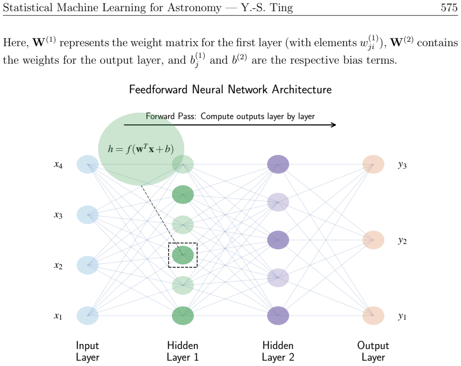
**Figure 15.3.** Figure 15.3: Architecture of a fully connected feedforward neural network, also known as a [PITH_FULL_IMAGE:figures/full_fig_p575_15_3.png]

**Figure 15.4.** Figure 15.4: Comparison between classical statistical learning theory and the modern dou [PITH_FULL_IMAGE:figures/full_fig_p579_15_4.png]

**Figure 15.5.** Figure 15.5: Stochastic Gradient Descent (SGD) with different learning rates navigating a [PITH_FULL_IMAGE:figures/full_fig_p584_15_5.png]

**Figure 15.6.** Figure 15.6: Common learning rate schedules used in neural network training. The left panel [PITH_FULL_IMAGE:figures/full_fig_p585_15_6.png]

**Figure 15.7.** Figure 15.7: Comparison of Stochastic Gradient Descent (SGD, left) and Adaptive Moment [PITH_FULL_IMAGE:figures/full_fig_p587_15_7.png]

**Figure 15.8.** Figure 15.8: Visualization of gradient approximation using the finite difference method for a [PITH_FULL_IMAGE:figures/full_fig_p593_15_8.png]

**Figure 15.9.** Figure 15.9: Computational graph for a simple neural network showing the forward pass with [PITH_FULL_IMAGE:figures/full_fig_p595_15_9.png]

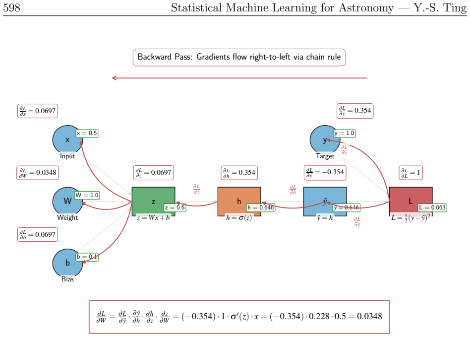
**Figure 15.10.** Figure 15.10: Visualization of the backward pass in backpropagation, showing how gradients [PITH_FULL_IMAGE:figures/full_fig_p598_15_10.png]

**Figure 15.11.** Figure 15.11: Comparison of forward mode and backward mode gradient calculation meth [PITH_FULL_IMAGE:figures/full_fig_p600_15_11.png]

**Figure 15.12.** Figure 15.12: Schematic comparison of Convolutional Neural Networks (CNNs) and Trans [PITH_FULL_IMAGE:figures/full_fig_p605_15_12.png]

**Figure 15.13.** Figure 15.13: Comparison of sigmoid and ReLU activation functions and their derivatives. [PITH_FULL_IMAGE:figures/full_fig_p609_15_13.png]

**Figure 15.14.** Figure 15.14: Visualization of superlinear versus non-superlinear functions. The light red [PITH_FULL_IMAGE:figures/full_fig_p611_15_14.png]

**Figure 15.15.** Figure 15.15: Visualization of the dropout technique for neural networks. The left panel [PITH_FULL_IMAGE:figures/full_fig_p614_15_15.png]

**Figure 15.16.** Figure 15.16: Schematic illustration of the “grokking” phenomenon in neural networks. The [PITH_FULL_IMAGE:figures/full_fig_p621_15_16.png]

**Figure 15.17.** Figure 15.17: Schematic illustration comparing foundation models with few-shot learning [PITH_FULL_IMAGE:figures/full_fig_p623_15_17.png]

**Figure 15.18.** Figure 15.18: Architecture of an autoencoder neural network for nonlinear dimension reduc [PITH_FULL_IMAGE:figures/full_fig_p628_15_18.png]

**Figure 15.19.** Figure 15.19: Comparison of linear and nonlinear dimensionality reduction techniques using [PITH_FULL_IMAGE:figures/full_fig_p630_15_19.png]

**Figure 15.20.** Figure 15.20: Encoder-decoder architectures for transformations between data domains. (a) [PITH_FULL_IMAGE:figures/full_fig_p635_15_20.png]

**Figure 15.21.** Figure 15.21: Comparing deterministic and probabilistic approaches to modeling one-to [PITH_FULL_IMAGE:figures/full_fig_p637_15_21.png]

**Figure 15.22.** Figure 15.22: Architecture of a Mixture Density Network (MDN) for modeling conditional [PITH_FULL_IMAGE:figures/full_fig_p640_15_22.png]

**Figure 15.23.** Figure 15.23: Visualization of normalizing flows showing the gradual transformation between [PITH_FULL_IMAGE:figures/full_fig_p644_15_23.png]

**Figure 15.24.** Figure 15.24: Visualization of diffusion models showing the gradual addition of noise to [PITH_FULL_IMAGE:figures/full_fig_p646_15_24.png]

**Figure 15.25.** Figure 15.25: Visualization of Simulation-Based Inference (SBI) showing the relationship [PITH_FULL_IMAGE:figures/full_fig_p650_15_25.png]

Discussion (0). Sign in to comment.

Forward citations

Cited by 1 Pith paper

Reviewed papers in the Pith corpus that reference this work. Sorted by Pith novelty score. Full citation record

Anchoring Stellar Age Indicators: A Cross-Calibration of [C/N] and Gyrochronology Ages via the Age-Velocity-Dispersion Relation
astro-ph.SR 2025-06 conditional novelty 6.0 of 10

After anchoring gyrochronology and [C/N] ages to the same age-velocity-dispersion relation, the two methods give consistent ages once small offsets are subtracted, and their valid parameter spaces are mapped.

Reference graph

Works this paper leans on

20 extracted references · 4 canonical work pages · cited by 1 Pith paper

[10]

G. E. Hinton, N. Srivastava, A. Krizhevsky, I. Sutskever, and R. R. Salakhutdinov. Im- proving neural networks by preventing co-adaptation of feature detectors. arXiv preprint arXiv:1207.0580. 670 Statistical Machine Learning for Astronomy — Y.-S. Ting J. Ho, A. Jain, and P. Abbeel. Denoising diffusion probabilistic models. arXiv preprint arXiv:2006.11239...

arXiv 2006
[14]

Nakkiran, G

P. Nakkiran, G. Kaplun, Y. Bansal, T. Yang, B. Barak, and I. Sutskever. Deep double descent: where bigger models and more data hurt. arXiv preprint arXiv:1912.02292 . R. M. Neal. Bayesian learning for neural networks . Springer,

arXiv 1912
[17]

D. J. Rezende and S. Mohamed. Variational inference with normalizing flows. arXiv preprint arXiv:1505.05770. H. Robbins and S. Monro. A stochastic approximation method. Annals of Mathematical Statistics, 22(3):400–407,

arXiv
[1878]

Adlam and J

B. Adlam and J. Pennington. Understanding double descent requires a fine-grained bias- variance decomposition. arXiv preprint arXiv:2011.03321 . H. Akaike. A new look at the statistical model identification. IEEE Transactions on Auto- matic Control, 19(6):716–723,

arXiv 2011
[1934]

Bommasani, D

R. Bommasani, D. A. Hudson, E. Adeli, R. Altman, S. Arora, S. von Arx, M. S. Bern- stein, J. Bohg, A. Bosselut, E. Brunskill, E. Brynjolfsson, S. Buch, D. Card, R. Castellon, N. Chatterji, A. Chen, K. Creel, J. Q. Davis, D. Demszky, C. Donahue, M. Doumbouya, E. Durmus, S. Ermon, J. Etchemendy, K. Ethayarajh, L. Fei-Fei, C. Finn, T. Gale, L. Gille- spie, K...

arXiv
[1963]

A. G. de G. Matthews, M. Rowland, J. Hron, R. E. Turner, and Z. Ghahramani. Gaussian process behaviour in wide deep neural networks. arXiv preprint arXiv:1804.11271 . P. McCullagh and J. A. Nelder. Generalized linear models (2nd ed.) . Chapman and Hall,

arXiv
[1971]

Zellner and P

A. Zellner and P. E. Rossi. Bayesian analysis of dichotomous quantal response models. Journal of Econometrics , 25(3):365–393, 1984

work page 1984
[1973]

Durkan, A

C. Durkan, A. Bekasov, I. Murray, and G. Papamakarios. Neural spline flows.arXiv preprint arXiv:1906.04032. G. M. Eadie, J. S. Speagle, J. Cisewski-Kehe, D. Foreman-Mackey, D. Huppenkothen, D. E. Jones, A. Springford, and H. Tak. Practical guidance for bayesian inference in astronomy. arXiv preprint arXiv:2302.04703 . C. Eckart and G. Young. The approxima...

arXiv 1906

Show all 20 references

[1977]

D. P. Kingma and M. Welling. Auto-encoding variational bayes. arXiv preprint arXiv:1312.6114. S. Kullback and R. A. Leibler. On information and sufficiency. Annals of Mathematical Statistics, 22(1):79–86,

arXiv
[1978]

Papamakarios, D

G. Papamakarios, D. C. Sterratt, and I. Murray. Sequential neural likelihood: fast likelihood- free inference with autoregressive flows. arXiv preprint arXiv:1805.07226 . K. Pearson. Iii. contributions to the mathematical theory of evolution. Philosophical Trans- actions of th...

arXiv
[1983]

Devlin, M.-W

J. Devlin, M.-W. Chang, K. Lee, and K. Toutanova. Bert: pre-training of deep bidirectional transformers for language understanding. arXiv preprint arXiv:1810.04805 . L. Devroye. Non-uniform random variate generation . Springer,

arXiv
[1984]

J. Geweke. Evaluating the accuracy of sampling-based approaches to the calculation of posterior moments. In: J. M. Bernardo, J. O. Berger, A. P. Dawid and A. F. M. Smith, Eds., Bayesian Statistics, Vol. 4, Clarendon Press, Oxford, 1992, pp. 169-193 ,

1992
[1987]

T. B. Brown, B. Mann, N. Ryder, M. Subbiah, J. Kaplan, P. Dhariwal, A. Neelakantan, P. Shyam, G. Sastry, A. Askell, S. Agarwal, A. Herbert-Voss, G. Krueger, T. Henighan, R. Child, A. Ramesh, D. M. Ziegler, J. Wu, C. Winter, C. Hesse, M. Chen, E. Sigler, M. Litwin, S. Gray, B. ...

2005 arXiv
[1990]

Jacot, F

A. Jacot, F. Gabriel, and C. Hongler. Neural tangent kernel: convergence and generalization in neural networks. arXiv preprint arXiv:1806.07572 . E. T. Jaynes. Probability theory: The logic of science . Cambridge University Press, Cam- bridge,

arXiv
[1992]

Qui˜ nonero-Candela and C

J. Qui˜ nonero-Candela and C. E. Rasmussen. A unifying view of sparse approximate gaussian process regression. Journal of Machine Learning Research , 6(65):1939–1959,

1939
[1995]

Ting 667 L

Statistical Machine Learning for Astronomy — Y.-S. Ting 667 L. Dinh, J. Sohl-Dickstein, and S. Bengio. Density estimation using real nvp. arXiv preprint arXiv:1605.08803. R. O. Duda, P. E. Hart, and D. G. Stork. Pattern classification (2nd ed.) . Wiley,

arXiv
[2003]

J. Wei, Y. Tay, R. Bommasani, C. Raffel, B. Zoph, S. Borgeaud, D. Yogatama, M. Bosma, D. Zhou, D. Metzler, E. H. Chi, T. Hashimoto, O. Vinyals, P. Liang, J. Dean, and W. Fe- dus. Emergent abilities of large language models. arXiv preprint arXiv:2206.07682 . C. K. I. Williams. ...

arXiv
[2005]

Y. Song, J. Sohl-Dickstein, D. P. Kingma, A. Kumar, S. Ermon, and B. Poole. Score- based generative modeling through stochastic differential equations. arXiv preprint arXiv:2011.13456. N. Srivastava, G. E. Hinton, A. Krizhevsky, I. Sutskever, and R. R. Salakhutdinov. Dropout: ...

2011 arXiv
[2006]

C. I. Bliss. The method of probits. Science, 79(2037):38–39,
[2020]

I. J. Goodfellow, J. Pouget-Abadie, M. Mirza, B. Xu, D. Warde-Farley, S. Ozair, A. Courville, and Y. Bengio. Generative adversarial networks. arXiv preprint arXiv:1406.2661 . D. S. Greenberg, M. Nonnenmacher, and J. H. Macke. Automatic posterior transformation for likelihood-f...

1905 arXiv

Pith tools

Reviewed August 7, 2026 · model on record in the stance chip above.

[1] [10]

G. E. Hinton, N. Srivastava, A. Krizhevsky, I. Sutskever, and R. R. Salakhutdinov. Im- proving neural networks by preventing co-adaptation of feature detectors. arXiv preprint arXiv:1207.0580. 670 Statistical Machine Learning for Astronomy — Y.-S. Ting J. Ho, A. Jain, and P. Abbeel. Denoising diffusion probabilistic models. arXiv preprint arXiv:2006.11239...

arXiv 2006

[2] [14]

Nakkiran, G

P. Nakkiran, G. Kaplun, Y. Bansal, T. Yang, B. Barak, and I. Sutskever. Deep double descent: where bigger models and more data hurt. arXiv preprint arXiv:1912.02292 . R. M. Neal. Bayesian learning for neural networks . Springer,

arXiv 1912

[3] [17]

D. J. Rezende and S. Mohamed. Variational inference with normalizing flows. arXiv preprint arXiv:1505.05770. H. Robbins and S. Monro. A stochastic approximation method. Annals of Mathematical Statistics, 22(3):400–407,

arXiv

[4] [1878]

Adlam and J

B. Adlam and J. Pennington. Understanding double descent requires a fine-grained bias- variance decomposition. arXiv preprint arXiv:2011.03321 . H. Akaike. A new look at the statistical model identification. IEEE Transactions on Auto- matic Control, 19(6):716–723,

arXiv 2011

[5] [1934]

Bommasani, D

R. Bommasani, D. A. Hudson, E. Adeli, R. Altman, S. Arora, S. von Arx, M. S. Bern- stein, J. Bohg, A. Bosselut, E. Brunskill, E. Brynjolfsson, S. Buch, D. Card, R. Castellon, N. Chatterji, A. Chen, K. Creel, J. Q. Davis, D. Demszky, C. Donahue, M. Doumbouya, E. Durmus, S. Ermon, J. Etchemendy, K. Ethayarajh, L. Fei-Fei, C. Finn, T. Gale, L. Gille- spie, K...

arXiv

[6] [1963]

A. G. de G. Matthews, M. Rowland, J. Hron, R. E. Turner, and Z. Ghahramani. Gaussian process behaviour in wide deep neural networks. arXiv preprint arXiv:1804.11271 . P. McCullagh and J. A. Nelder. Generalized linear models (2nd ed.) . Chapman and Hall,

arXiv

[7] [1971]

Zellner and P

A. Zellner and P. E. Rossi. Bayesian analysis of dichotomous quantal response models. Journal of Econometrics , 25(3):365–393, 1984

work page 1984

[8] [1973]

Durkan, A

C. Durkan, A. Bekasov, I. Murray, and G. Papamakarios. Neural spline flows.arXiv preprint arXiv:1906.04032. G. M. Eadie, J. S. Speagle, J. Cisewski-Kehe, D. Foreman-Mackey, D. Huppenkothen, D. E. Jones, A. Springford, and H. Tak. Practical guidance for bayesian inference in astronomy. arXiv preprint arXiv:2302.04703 . C. Eckart and G. Young. The approxima...

arXiv 1906