REVIEW 3 major objections 5 minor 4 cited by
Relaxation for massive particles: transport and causality
T0 review · 3 major / 5 minor · reviewed 2026-08-15 · deepseek-v4-flash
Pith's one-line read All first-order transport coefficients of a massive RTA gas are now known in closed form and remain positive for every mass.
desk verdict Solid analytic transport results for massive RTA, but Eq. (59) is dimensionally off by a factor T0 and the causal-cut interpretation is heuristic. read the letter →
The pith
A machine-rendered reading of the paper's core claim, the machinery that carries it, and where it could break.
The reading
What carries the argument
The load-bearing object is the retarded two-point correlator written as a double integral over energy, $u\in[0,1]$, and angle, $z\in[-1,1]$, as in Eq. (94), carrying the Maxwell-J\"uttner weight $\exp(-m/(T_0\sqrt{1-u^2}))$. The mass enters through the particle velocity $\xi=\sqrt{1-m^2/x^2}$, coupling the momentum integral to the angular integral so that the denominator $1-i\omega\tau_R+ik\tau_R z u$ has a continuum of zeros, generating a cut instead of a movable logarithmic branch point. The argument then extracts transport coefficients from the diffusive pole of this integral in the hydrodynamic limit, computes the discontinuity profile by the residue-style procedure of Appendix B, and defines $v_{\rm cut}$ as the threshold $\epsilon$ below which the discontinuity is exponentially suppressed.
What would settle it
Evaluate the exact diffusion constants, for instance Eq. (39) in $d=3$ or Eq. (A22) in $d=2$, at large $m/T_0$: if either $D$ or $D_{\rm sh}$ turns negative at any mass, the positivity claim fails. Separately, deform the angular integration contour $\xi_c$ in Eq. (94) and test whether the resulting correlator satisfies the usual causal analyticity conditions; a causal deformed-contour correlator with a different cut would refute the claimed indeformability.
Extended reading notes
Core claim
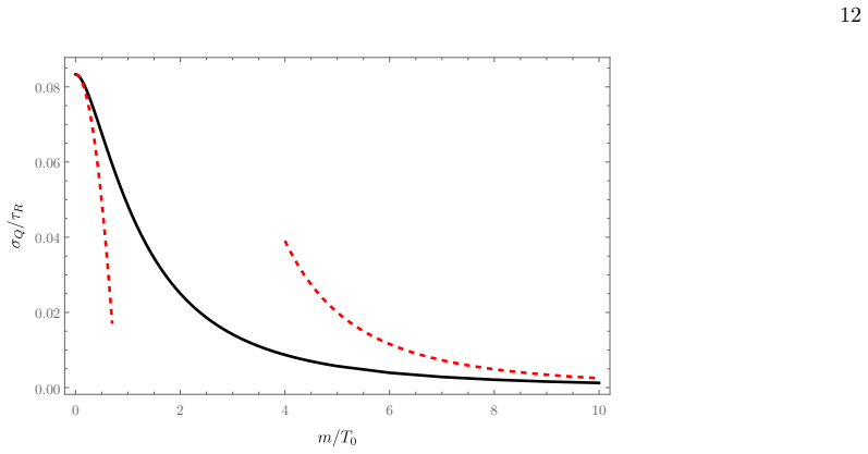
On the paper's own terms, the central discovery is that mass does not destabilize RTA hydrodynamics but reshapes its analytic structure. The diffusive-pole integral equations are solved in closed form: $D/\tau_R$ is a Meijer $G$-function combination in Eq. (32), $D_{\rm sh}/\tau_R$ in Eq. (39), the bulk viscosity in Eq. (50), the shear viscosity in Eq. (59), and the thermoelectric DC conductivity $\sigma_Q$ in Eq. (77); all remain positive for all masses and reduce correctly in the $m\to 0$ and $m\to\infty$ limits. In the complex frequency plane, finite mass turns the logarithmic branch cut of the massless theory into a straight cut between $\omega=\pm k-i/\tau_R$ that cannot be deformed, because the energy and angular integrations are coupled: deforming either contour removes a two-dimensional region from the domain of the correlator. The endpoints of this cut mark the maximal propagation speed, while the shape of the discontinuity along it defines a threshold criterion $v_{\rm cut}$ (Eq. (90)) for the effective ballistic lightcone, which is distinct from the mean or rms particle speed and from the speed of sound.
Load-bearing premise
The paper's unique straight cut rests on the assumption that the only physically admissible analytic continuation keeps both integration variables real, $u\in[0,1]$ and $z\in[-1,1]$; the paper notes that deformed contours may be inconsistent with causal correlators but does not prove that causality forces this particular contour.
Editorial extensions
If this is right
- For any $d\ge 2$, charge and shear diffusion constants are non-negative for all $m/T_0$; the earlier claimed instability in [31] is an artefact of extrapolating the small-mass expansion, and the exact expressions give $D/\tau_R\to 1/m$ at large mass.
- The sound channel is consistent with first-order hydrodynamics: the leading pole speed equals the equation-of-state speed of sound, and the attenuation $\Gamma_s$ is non-negative, with bulk viscosity matching the Kubo formula and Chapman-Enskog results.
- At finite mass the correlator's cut between $\pm k-i/\tau_R$ is undeformable, so the hydrodynamic pole eventually meets the cut at a finite wavenumber $k_*$ that grows with mass and dimension; in the massless theory the cut can be deformed to avoid the pole, so no such cutoff is forced.
- The discontinuity profile of the cut carries causal information: its endpoints give the maximum speed, namely the speed of light, while the criterion $v_{\rm cut}$ gives an effective lightcone that moves to smaller velocities as mass increases.
- The thermoelectric transport coefficients are parameterized by a single microscopic quantity, the DC conductivity $\sigma_Q$, with all other response fixed by thermodynamics and Ward identities.
Reading between the lines
- If the indeformability argument carries over to RTA with energy-dependent relaxation time or to weakly coupled massive field theories, one expects the same two-dimensional non-analytic region rather than a condensate of branch points; this is a testable extension of Section IV B, not established here.
- The $v_{\rm cut}$ criterion suggests an operational definition: in any system whose retarded correlator has a discontinuity tail, an effective lightcone speed can be extracted by thresholding the normalized discontinuity at a fixed small $\epsilon$; applying this to other channels could reveal whether $v_{\rm cut}$ is universal or channel-dependent.
- The exact positivity of all first-order coefficients for $d>1$ makes it plausible that higher-order RTA transport coefficients remain well-behaved in the massive theory, although the paper does not compute them beyond finding $\kappa=0$ and $\tau_\pi=\tau_R$ independent of mass.
Signed reviews
Editorial analysis
A structured set of objections, weighed in public.
Referee Report
Summary. The manuscript studies massive relativistic particles in the relaxation time approximation of kinetic theory at finite temperature and density. It derives closed-form expressions for the first-order transport coefficients—charge and shear diffusion constants D and D_sh, bulk viscosity ζ, shear viscosity η, and DC thermoelectric conductivity σ_Q—as functions of m/T0, using the variational/Kubo approach to retarded correlators. It also analyzes the analytic structure of the correlators, identifies a cut at Im ω = -1/τ_R between ω = ±k - i/τ_R, studies its discontinuity profile as a function of mass, and proposes a criterion (disc G = ε) that extracts an 'effective lightcone velocity' v_cut. The paper further claims to correct an instability reported in Ref. [31], showing positive diffusion coefficients for all masses in d>1, and discusses the indeformability of the cut at finite mass.
Significance. If the results hold, the paper provides a useful exact reference: all first-order transport coefficients of the massive RTA gas in closed form, with cross-checks against Kubo formulas, Ward identities, Chapman–Enskog results, and positivity/stability in arbitrary dimensions. The paper contains no fitted parameters in the transport coefficients and gives explicit analytic formulas (e.g., (32), (39), (50), (77)) that can be implemented directly. These strengths are offset by two caveats: the printed shear viscosity (59) is dimensionally inconsistent, and the claimed indeformability/uniqueness of the cut in Section IV B is argued heuristically rather than proven. The v_cut criterion also depends on an arbitrary threshold ε. The central positivity result is robust, but the 'complete analytic expressions' claim is not true as printed until Eq. (59) is corrected.
major comments (3)
- [III B 3, Eq. (59)] Equation (59) as printed is dimensionally inconsistent: the right-hand side has energy dimension four (τ_R times an integral scaling as T0^5), whereas the shear viscosity η has energy dimension three. The missing factor is 1/T0 in front of the integral, as is visible by comparing with Eq. (71) and with the required cross-check η = D_sh(ε0 + P0). At m=0, Eq. (59) gives η = 4τ_R T0^5/(5π^2) instead of 4τ_R T0^4/(5π^2). Since Eq. (59) is one of the five closed-form transport coefficients advertised in the abstract, the central claim is not true as printed; any reader implementing (59) obtains viscosities off by a factor of T0. The positivity/stability conclusion is unaffected because D and D_sh are ratios of positive integrals, but the formula must be corrected before the manuscript can be accepted.
- [IV B, Eq. (94)] The claim that the cut is undeformable and unique is not established. The argument that deforming the angular contour removes a two-dimensional region and 'may be inconsistent' with causal correlators does not prove that the real-u, real-z contour is forced by causality; the sentence 'this implies a unique choice of the cut' overstates the result. As the authors themselves note, other analytic continuations might be physically allowed, and the discussion of the pole merging with the cut at k_* depends on this choice. The paper should either provide a proof from analyticity/causality of the retarded correlator or explicitly present the straight cut as a preferred convention rather than as a uniqueness statement.
- [IV A, Eq. (90)] The definition of v_cut via disc G = ε depends on an arbitrarily chosen threshold ε, and no physical principle selects a value of ε. The numerical demonstrations use ε = 10^-3 without showing that v_cut is stable or meaningful under changes of ε, and the same ε-dependence enters the toy model expression (B16). As it stands, the 'extraction of physical information from the discontinuity profile' is convention-dependent, which weakens the claim that v_cut encodes an effective lightcone. The authors should quantify the ε-dependence and either justify a canonical choice or soften the interpretation.
minor comments (5)
- [II A, Eqs. (17)–(20)] The symbol m is used both for the dimensionful mass (in the integration limits and in quantities such as ε0 and P0) and for the dimensionless ratio m/T0 (in the Bessel functions and the Meijer-G expressions). This is confusing; a separate notation such as m̂ = m/T0 would improve readability.
- [Abstract and Section II A] The abstract advertises 'finite density', but the thermodynamic expressions in Section II A are derived 'in the absence of chemical potential'. The authors should clarify whether finite density means nonzero n0 at zero chemical potential or whether µ0 ≠ 0 results are included, since the thermoelectric section later uses n0 and s0.
- [Figure 1 caption] The caption writes the cut endpoints as ω = ±ck − i/τ_R, while the text and Eq. (95) use ±k − i/τ_R with c implicitly set to unity. The speed of light c should be defined or omitted to avoid confusion.
- [IV B, k_* discussion] The statement that the cutoff wavevector k_* (where the diffusive pole reaches the cut) increases with mass and spatial dimension is made without presenting the corresponding formula or numerical evidence, making it difficult to verify.
- [Appendix B, Eq. (B16)] In the toy-model definition of v_cut, the result depends on ε through both log ε and ε itself; using a different normalization of the discontinuity profile would change v_cut. It would be helpful to state explicitly that v_cut is a threshold-dependent quantity and to give its behavior for representative ε values.
Circularity Check
No significant circularity: transport coefficients are computed directly from RTA kinetic theory, the vcut condition is explicitly definitional, and the sole self-citation is not load-bearing.
full rationale
The central transport results — D(m) in Eq. (32), D_sh(m) in Eq. (39), ζ/(ε0+P0) in Eq. (50), η in Eq. (59), and σ_Q in Eq. (77) — are obtained by expanding pole equations derived from the linearized RTA Boltzmann equation (11) and matching conditions (13), or by direct Kubo integrals of retarded correlators. The inputs are the Maxwell–Jüttner equilibrium distribution, τ_R, m, and T0; no parameter is fitted to the outputs. The only self-citation, [24], supplies conventions and the standard massless contour-deformation discussion, but the massive transport integrals and positivity statements are evaluated in this paper and are cross-checked against external Chapman–Enskog results [46] and Kubo formulas, so [24] is not load-bearing. The vcut criterion in Eq. (90) is explicitly proposed as a definition ('We propose a condition ... which defines the velocity vcut'); a convention with an arbitrary ϵ is not a derived prediction reduced to its input. Section IV B's indeformability claim rests on an unproven preference for real u,z contours, so the uniqueness assertion is a gap rather than a circular reduction. Eq. (59) also appears dimensionally inconsistent as printed (missing a factor 1/T0), but that is a transcription error, not a fitted parameter renamed as a prediction. Therefore no circular step is present.
Assumptions & free parameters
free parameters (1)
- threshold epsilon in vcut criterion =
epsilon = 10^-3 in the figures (arbitrary)
assumptions (5)
- domain assumption The RTA Boltzmann equation with constant tau_R approximates the collision kernel with a single relaxation time and yields the analytic structure of the true kinetic theory.
- domain assumption The equilibrium distribution is the Maxwell-Juettner distribution and linear response around it is valid.
- ad hoc to paper The preferred analytic continuation for the massive double integral keeps u and z real, fixing the cut between +/- k - i/tau_R.
- ad hoc to paper The vcut criterion disc G = epsilon is a meaningful definition of effective lightcone speed.
- standard math Standard results from complex analysis, residue theorem, Meijer G and hypergeometric functions are used without proof.
invented entities (1)
-
effective lightcone velocity vcut
Cite this review
Pith. "Pith review of Relaxation for massive particles: transport and causality." pith.science (2026). https://pith.science/paper/YBPXPMCN
@misc{pith2026250615531,
  author       = {Pith},
  title        = {Pith review of: Relaxation for massive particles: transport and causality},
  year         = {2026},
  howpublished = {\url{https://pith.science/paper/YBPXPMCN}},
  note         = {Machine review of arXiv:2506.15531}
}
read the original abstract
Correlators at finite density and temperature encode important information about a physical system, such as transport and causality. For a massive gas of particles in the relaxation time approximation of kinetic theory, we provide complete analytic results for all first order transport coefficients, including thermoelectric coefficients. We demonstrate the first complete picture of the complex structure of the correlators as a function of mass, providing an interpretation in terms of the causal structure of lightcones. We provide a simple criterion to extract the effective lightcone velocity from the cut of the retarded correlator.
Figures


Figures from the paper (11 more)


Forward citations
Cited by 4 Pith papers
-
The Lorentzian geometry of relaxation
Causality forces purely relaxational dispersion relations to follow spacelike trajectories on the Lorentzian {iω,ik} plane, producing universal bounds on diffusivity, viscosity, time-dilation deviations, and hydrodyna...
-
How Lorentz boosts reshape relaxation spectra
Under an Onsager-type symmetry, boosted k=0 non-hydrodynamic relaxation rates of a relativistic fluid are bounded by a(1-v)/γ ≤ iω' ≤ b/[γ(1-v)] in terms of rest-frame bounds a,b and boost speed v.
-
Imaging non-hydrodynamic modes with jet wakes
In the long-wavelength limit, jet-wake angular moments with ℓ≥3 vanish in hydrodynamics and directly image the non-hydrodynamic relaxation spectrum of the medium.
-
Order-reversed Kubo formulas in relativistic kinetic theory
In a simplified relativistic gas model, eight alternative Kubo formulas for viscosity give identical values, supporting the new order-of-limits method.
Reference graph
Works this paper leans on
-
[31]
Quasi-particle hydrodynamics with momentum-dependent relaxation time
A. Mukherjee, S. Bhadury, and P. Singha, (2025), arXiv:2504.11572 [hep-ph]
work page Pith review arXiv 2025
-
[1]
Integrals of functions with a branch cut 19
-
[2]
Discontinuity profile, branch cuts and branch points 19
Shear diffusion 18 B. Discontinuity profile, branch cuts and branch points 19
-
[3]
Thermoelectric transport 10 IV
Tensor channel 10 C. Thermoelectric transport 10 IV. Non-hydrodynamic modes 12 A. Physical interpretation of analytic structure in the massive case 13 B. Indeformability of the cut at finite mass 15 V. Conclusion 16 Acknowledgments 17 A. Massive transport in arbitrary dimensions 17
-
[4]
Complex integrals of meromorphic functions 22 References 24 I. INTRODUCTION The emergence of collective phenomena from microscopic dynamics has been a key research frontier, leading to robust characterization of near- and non-equilibrium physics. To that end, an often utilized microscopic description ∗ matej.bajec@fmf.uni-lj.si † alexander.soloviev@fmf.un...
arXiv 2025
-
[5]
Shear channel We perform a similar derivation of the diffusion constant equation as in the charge diffusion case. The simplest case is the shear diffusion channel, schematically denoted with δT 0⊥, where⊥ is one of the transverse components to our chosen axis aligned with the wave vector k. For concreteness, we fix the transverse direction to ⊥=y; other c...
-
[6]
Sound channel We now consider the longitudinal channel, i.e. the sound. Here we only turn on sources that induce δT and δuz, since ki∝δi z. In order to solve the self–consistency condition and obtain the analytic structure of the correlators in this channel, one must solve two coupled linear equations for the perturbations δT and δuz or equivalently for δ...
-
[7]
Tensor channel To determine the shear viscosity, it is enough to turn on just the metric perturbation, δgxy(ω,k ). This does not induce any change in the macroscopic variables ( δT , δui), so there is no need to solve the matching conditions. The correlator is given by the following integral Gxy,xy =− δ δgxy Z d3p (2π)3 pxpy p0 δf, (54) =− Z d3p (2π)3 pxp...
Show all 69 references
-
[8]
Charge diffusion We first consider the charge diffusion in arbitrary dimensions by focusing on the diffusive pole given by Eq. (28). The integral I00 can be generalized to arbitrary dimension: I00 (d) = Z dΩ(d) Ω(d) 1 1 +τR (−iω +iξk· v), (A1) where dΩ(d) is the d–dimensional ...
-
[9]
For the sake of concreteness let us pick p⊥ to be aligned along the x2 axis and denote it py in order to not confuse it with the square of the momentum
Shear diffusion Start with the solution of the linearized Boltzmann equation in the case of external metric perturbation: δf = f0 T0 piδui + δT T0 p0−τRΓ0 αβp0˜vα˜vβ 1 +τR (−iω +iξk· v) (A15) = f0 T0 p⊥δu⊥−τRΓ0 αβ˜vα˜vβ 1 +τR(−iω +ikξ cosθ1), (A16) 19 where we turned off the p...
-
[10]
Example 1
Integrals of functions with a branch cut In this appendix we showcase the general procedure to describe the analytic structure of an integral of a function with branch points via several examples of increasing complexity. Example 1. We start with the simplest example 7 F (ω)≡ ...
-
[11]
Identify the ‘furthermost’ branch point ωbp, meaning the branch point that shares the branch cut with all the other branch points (when varying the integration parameter)
Choose a branch cut of the integrand and consider all of its branch points (and cuts) as the integration parameter varies. Identify the ‘furthermost’ branch point ωbp, meaning the branch point that shares the branch cut with all the other branch points (when varying the integr...
-
[12]
In our case, the limiting value of u is given by −k q 1−u2 δ =ε =⇒uδ = r 1− δ2 k2
Fix a value δ >0 and calculate the interval of u for which the branch point of the integrand is still less than δ away fromωbp. In our case, the limiting value of u is given by −k q 1−u2 δ =ε =⇒uδ = r 1− δ2 k2. (B12) 8 One can reinstate a finite τR by making a substitution ω 7...
-
[13]
(B14) The final step is a trivial transformation from δ to ω
Finally integrate the discontinuity (in this case 2 πi because of the logarithm) along the calculated interval: discF (ω;k,m ) ω=ωbp−δ = 2πim Z uδ= q 1−δ2 k2 0 du u2e−m T0 1 u (B13) = 2πiT 0 exp −m T0 1q 1− δ2 k2 . (B14) The final step is a trivial transformation from δ ...
-
[14]
For the sake of completeness we restate the origin of the branch cut structure in RTA kinetic theory
Complex integrals of meromorphic functions Here we review and expand upon the discussion from Appendix A found in [24], which supports the discussion in Section IV B. For the sake of completeness we restate the origin of the branch cut structure in RTA kinetic theory. 23 0 10 ...
-
[15]
Pitaevskii and E
L. Pitaevskii and E. Lifshitz, Physical Kinetics: Volume 10 , let. 10 (Butterworth-Heinemann, 2012)
2012
-
[16]
de Groot, W
S. de Groot, W. van Leeuwen, and C. van Weert, Relativistic Kinetic Theory (North-Holland Publishing Company, Amsterdam, Netherlands, 1980)
1980
-
[17]
Anderson and H
J. Anderson and H. Witting, Physica 74, 466 (1974)
1974
-
[18]
Liboff, Kinetic Theory (Springer-Verlag, New York, USA, 2003)
R. Liboff, Kinetic Theory (Springer-Verlag, New York, USA, 2003)
2003
-
[19]
Grozdanov, N
S. Grozdanov, N. Kaplis, and A. O. Starinets, JHEP 07, 151 (2016), arXiv:1605.02173 [hep-th]
2016 arXiv
- [20]
-
[21]
Florkowski, R
W. Florkowski, R. Ryblewski, and M. Strickland, Nucl. Phys. A 916, 249 (2013), arXiv:1304.0665 [nucl-th]
2013 arXiv
-
[22]
Florkowski, R
W. Florkowski, R. Ryblewski, and M. Strickland, Phys. Rev. C 88, 024903 (2013), arXiv:1305.7234 [nucl-th]. 25 0.0 0.2 0.4 0.6 0.8 1.0 0.0 0.2 0.4 0.6 0.8 1.0 Figure 14. Absolute value of the normalized discontinuity of the integral (B21) for different values of mass m as a fun...
2013 arXiv
-
[23]
Florkowski, E
W. Florkowski, E. Maksymiuk, R. Ryblewski, and M. Strickland, Phys. Rev. C 89, 054908 (2014), arXiv:1402.7348 [hep-ph]
2014 arXiv
-
[24]
Kurkela and U
A. Kurkela and U. A. Wiedemann, Eur. Phys. J. C 79, 776 (2019), arXiv:1712.04376 [hep-ph]
2019 arXiv
-
[25]
Kurkela, U
A. Kurkela, U. A. Wiedemann, and B. Wu, Eur. Phys. J. C 79, 965 (2019), arXiv:1905.05139 [hep-ph]
2019 arXiv
-
[26]
D. Dash, S. Bhadury, S. Jaiswal, and A. Jaiswal, Phys. Lett. B 831, 137202 (2022), arXiv:2112.14581 [nucl-th]
2022 arXiv
-
[27]
V. E. Ambrus, S. Schlichting, and C. Werthmann, Phys. Rev. D 107, 094013 (2023), arXiv:2211.14379 [hep-ph]
2023 arXiv
- [28]
-
[29]
Hu, (2024), arXiv:2409.05131 [hep-ph]
J. Hu, (2024), arXiv:2409.05131 [hep-ph]
2024
-
[30]
S. K. Singh, S. Bhadury, M. Kurian, and V. Chandra, (2025), arXiv:2501.17442 [hep-ph]
2025 arXiv
-
[32]
Blaizot and L
J.-P. Blaizot and L. Yan, Phys. Rev. C 104, 055201 (2021), arXiv:2106.10508 [nucl-th]
2021 arXiv
-
[33]
Aniceto, J
I. Aniceto, J. Noronha, and M. l. Spal´ ınski, Phys. Rev. D 111, 076025 (2025), arXiv:2401.06750 [nucl-th]
2025 arXiv
-
[34]
V. E. Ambrus, E. Moln´ ar, and D. H. Rischke, Phys. Rev. D 106, 076005 (2022), arXiv:2207.05670 [nucl-th]
2022 arXiv
-
[35]
Jaiswal, J.-P
S. Jaiswal, J.-P. Blaizot, R. S. Bhalerao, Z. Chen, A. Jaiswal, and L. Yan, Phys. Rev. C 106, 044912 (2022), arXiv:2208.02750 [nucl-th]
2022 arXiv
-
[36]
V. E. Ambru¸ s, E. Moln´ ar, and D. H. Rischke, Phys. Rev. D109, 076001 (2024), arXiv:2311.00351 [nucl-th]
2024 arXiv
-
[37]
Ochsenfeld and S
S. Ochsenfeld and S. Schlichting, JHEP 09, 186 (2023), arXiv:2308.04491 [hep-th]
2023 arXiv
-
[38]
Bajec, S
M. Bajec, S. Grozdanov, and A. Soloviev, JHEP 08, 065 (2024), arXiv:2403.17769 [hep-th]
2024 arXiv
- [39]
-
[40]
G. S. Rocha and G. S. Denicol, (2025), arXiv:2505.14823 [nucl-th]
2025
-
[41]
Dusling and T
K. Dusling and T. Sch¨ afer, Phys. Rev. C85, 044909 (2012), arXiv:1109.5181 [hep-ph]
2012 arXiv
-
[42]
A. Das, H. Mishra, and R. K. Mohapatra, Phys. Rev. D 102, 014030 (2020), arXiv:2004.04665 [hep-ph]
2020 arXiv
-
[43]
Zebarjadi, S
M. Zebarjadi, S. E. Rezaei, M. S. Akhanda, and K. Esfarjani, Phys. Rev. B 103, 144404 (2021)
2021
- [44]
- [45]
- [46]
-
[47]
Grozdanov, A
S. Grozdanov, A. Lucas, and N. Poovuttikul, Phys. Rev. D 99, 086012 (2019), arXiv:1810.10016 [hep-th]
2019 arXiv
-
[48]
M. P. Heller, A. Serantes, M. Spali´ nski, and B. Withers, Phys. Rev. Lett. 130, 261601 (2023), arXiv:2212.07434 [hep-th]
2023 arXiv
-
[49]
M. P. Heller, A. Serantes, M. Spali´ nski, and B. Withers, Nature Phys. 20, 1948 (2024), arXiv:2305.07703 [hep-th]
2024 arXiv
-
[50]
Gavassino, M
L. Gavassino, M. M. Disconzi, and J. Noronha, Phys. Rev. Lett. 132, 162301 (2024), arXiv:2307.05987 [hep-th]
2024 arXiv
-
[51]
S. A. Hartnoll and S. P. Kumar, JHEP 12, 036 (2005), arXiv:hep-th/0508092
2005 arXiv
-
[52]
G. S. Rocha, I. Danhoni, K. Ingles, G. S. Denicol, and J. Noronha, Phys. Rev. D 110, 076003 (2024), arXiv:2404.04679 [nucl-th]
2024 arXiv
-
[53]
Casalderrey-Solana, S
J. Casalderrey-Solana, S. Grozdanov, and A. O. Starinets, Phys. Rev. Lett. 121, 191603 (2018), arXiv:1806.10997 [hep-th]
2018 arXiv
-
[54]
Grozdanov and A
S. Grozdanov and A. O. Starinets, JHEP 04, 080 (2019), arXiv:1812.09288 [hep-th]
2019 arXiv
- [55]
-
[56]
Gursoy, E
U. Gursoy, E. Kiritsis, and F. Nitti, JHEP 02, 019 (2008), arXiv:0707.1349 [hep-th]
2008 arXiv
-
[57]
Betzios, U
P. Betzios, U. G¨ ursoy, M. J¨ arvinen, and G. Policastro, Phys. Rev. D97, 081901 (2018), arXiv:1708.02252 [hep-th]
2018 arXiv
-
[58]
I. S. Gradshteyn, I. M. Ryzhik, D. Zwillinger, and V. Moll, Table of integrals, series, and products; 8th ed. (Academic 26 Press, Amsterdam, 2015)
2015
- [59]
-
[60]
Hattori, M
K. Hattori, M. Hongo, and X.-G. Huang, Symmetry 14, 1851 (2022), arXiv:2207.12794 [hep-th]
2022 arXiv
-
[61]
Cercignani and G
C. Cercignani and G. M. Kremer, The Relativistic Boltzmann Equation: Theory and Applications (Birkh¨ auser Basel, 2002)
2002
-
[62]
S. A. Hartnoll, P. K. Kovtun, M. Muller, and S. Sachdev, Phys. Rev. B 76, 144502 (2007), arXiv:0706.3215 [cond-mat.str- el]
2007 arXiv
-
[63]
S. A. Hartnoll, A. Lucas, and S. Sachdev, (2016), arXiv:1612.07324 [hep-th]
2016 arXiv
-
[64]
Kurkela, U
A. Kurkela, U. A. Wiedemann, and B. Wu, Eur. Phys. J. C 79, 759 (2019), arXiv:1805.04081 [hep-ph]
2019 arXiv
- [65]
-
[66]
Bazow, G
D. Bazow, G. S. Denicol, U. Heinz, M. Martinez, and J. Noronha, Phys. Rev. Lett. 116, 022301 (2016)
2016
-
[67]
Kurkela, A
A. Kurkela, A. Mukhopadhyay, F. Preis, A. Rebhan, and A. Soloviev, JHEP 08, 054 (2018), arXiv:1805.05213 [hep-ph]
2018 arXiv
-
[68]
Abramowitz and I
M. Abramowitz and I. Stegun, Handbook of mathematical functions with formulas, graphs, and mathematical tables (Dover, New York, 1964)
1964
-
[69]
L. V. Ahlfors, Complex Analysis , 2nd ed. (McGraw-Hill Book Company)
Reviewed August 15, 2026 · model on record in the stance chip above.
Discussion (0). Continue with ORCID to comment.