REVIEW 3 major objections 5 minor 43 references
Anomalous Bulk Current in Quantum Hall Systems with an Expanding Edge
T0 review · 3 major / 5 minor · reviewed 2026-08-06 · deepseek-v4-flash
Pith's one-line read An expanding quantum Hall edge produces a bulk energy current that exactly cancels the Hawking-like edge flux, so the total system conserves energy and momentum.
desk verdict Bulk current calculation is real and worth taking seriously, but the exact bulk-edge cancellation is proven only for an idealized translation-invariant profile, and the trace-anomaly factor of two needs fixing. read the letter →
The pith
A machine-rendered reading of the paper's core claim, the machinery that carries it, and where it could break.
The reading
What carries the argument
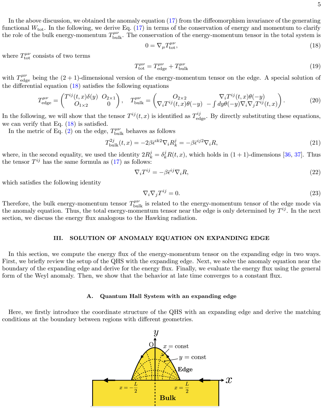
The load-bearing object is the (2+1)-dimensional gravitational Chern-Simons action with coefficient $\beta=c_-/96\pi$, which is what the gapped bulk contributes after the edge modes are integrated out. Its variation produces the bulk stress tensor $T^{\mu\nu}_{\rm bulk}$ and the Bardeen-Zumino boundary polynomial $P^{ij}$; the latter converts the consistent edge anomaly into the covariant anomaly equation, implementing anomaly inflow. On the expanding edge, the conformal factor $\omega(t,x)=1/\cos(Ht)$ in the middle region and the matching function $\Phi[x]=\int_0^x dy\,e^{\Theta(y)}$ encode the de Sitter-like geometry, and the Schwarzian derivative $\mathrm{Sch}[f,x^+_{III}]$ of the coordinate map between flat regions supplies the flux. In the bulk, the metric $ds^2=a^2(t,y)\eta_{ij}dx^idx^j+dy^2$ with $a^2=(\omega(t)^2-1)f(y)+1$ and a smooth profile $f(y)$ carries the energy-current calculation that yields Eq. (73).
What would settle it
Compute $\int_{-\infty}^0 dy\,T^{01}_{\rm bulk}$ in the full three-region metric of Eq. (24), where $\omega(t,x)$ depends on $x$ and the expansion is localized in a strip of width $L$, rather than in the translation-invariant proxy of Eq. (69); if the integral differs from $-c_-H^2/(48\pi)$ or depends on $L$, $n$, or time, the claimed exact compensation is false. A simpler numerical test is to repeat the integral with an interpolation function that violates $f'(0)=0$ and check whether the result shifts.
Extended reading notes
Core claim
The central discovery is that the covariant gravitational anomaly on the expanding edge, $\nabla_i T_{\rm cov}^{ij}=-\beta\bar{\epsilon}^{ij}\nabla_i R$, is induced by anomaly inflow from the bulk, and that solving this anomaly equation gives the edge energy flux $T^{III}_{++}=2\beta H^2\left[1-(\partial x^+_I/\partial x^+_{III})^2\right]$, which approaches $c_-H^2/(48\pi)$ at late times, matching a Gibbons-Hawking thermal flux. The new step is the bulk side: for a translation-invariant metric that interpolates smoothly between edge and flat bulk, the integrated bulk energy current $\int_{-\infty}^0 dy\,T^{01}_{\rm bulk}$ equals $-c_-H^2/(48\pi)$ independent of time and of the interpolation profile, while the total system remains energy-momentum conserving. The paper concludes that the total energy flux parallel to the edge is quantized and the edge anomaly is exactly compensated by the bulk.
Load-bearing premise
The exact cancellation is derived for a simplified edge that is identical at every point along its direction and only varies into the bulk; the actual localized expanding segment used to produce the Hawking-like flux does not have that simplified form, and the cancellation could fail there.
Editorial extensions
If this is right
- The Hawking-like edge flux from an expanding quantum Hall edge is not a leak: it is exactly balanced by an opposite bulk current, so the total system conserves energy and momentum.
- The integrated bulk current $\int dy\,T^{01}_{\rm bulk}=-c_-H^2/(48\pi)$ is universal in the studied profile class, being independent of time and of which smooth interpolation is used, making it a candidate quantized observable.
- The covariant form of the edge gravitational anomaly follows directly from anomaly inflow in this setup, connecting the expanding-edge geometry to the standard bulk-boundary correspondence.
- At late times the edge flux coincides with the chiral thermal flux at the Gibbons-Hawking temperature $T_{\rm GH}=H/2\pi$, so the expanding edge can serve as a condensed-matter analog of de Sitter radiation.
Reading between the lines
- If the exact compensation survives in the full localized, $x$-dependent edge metric, then any experiment that detects the edge Hawking-like flux should also detect a counterpropagating energy current in the bulk, which could serve as a direct falsification test.
- The universality in $n$ suggests the integrated bulk current may be a topological invariant of the anomaly-inflow structure, protected against details of how the edge is smoothed into the bulk; testing asymmetric or non-smooth profiles would sharpen this.
- The same covariant-anomaly machinery could be applied to other time-dependent boundaries, such as a contracting edge or a periodically modulated boundary, predicting analogous bulk compensation currents.
- The paper leaves the physical meaning of $T^{12}_{\rm bulk}$ open; a natural next step is to connect this shear-stress component to momentum exchanges or to measurable heating at the interface.
Editorial analysis
A structured set of objections, weighed in public.
Referee Report
Summary. The paper studies a (2+1)-dimensional quantum Hall system with an expanding edge, modeled by a curved metric that interpolates between a flat bulk and a de Sitter-like edge. It derives the covariant gravitational anomaly on the edge from anomaly inflow of a bulk gravitational Chern-Simons term, solves the anomaly equation to obtain an energy flux analogous to Hawking radiation, and reproduces the same flux via a Weyl-anomaly / Schwarzian-derivative computation. It then computes the bulk energy-momentum tensor for two spatial profile functions and claims that the integrated bulk energy current parallel to the edge is quantized and exactly cancels the edge flux. The paper includes analytic formulas for the bulk stress components and an appendix proving the equivalence of the two edge-flux derivations.
Significance. If the bulk-edge cancellation result were established in full generality, it would provide a concrete condensed-matter realization of gravitational anomaly inflow with an explicit bulk current compensating the edge anomaly, which is a valuable contribution. The paper has real strengths: the derivation of the covariant anomaly from the Chern-Simons boundary term is standard and clearly presented; Appendix C gives an independent analytical proof that the Schwarzian-derivative formula equals the anomaly-equation result; and Appendix D supplies explicit closed-form expressions for the bulk stress components for two profile families. The main new claim, however, is the exact compensation of the edge flux by the integrated bulk current, and that claim is currently demonstrated only for a restricted homogeneous proxy geometry and an idealized sharp profile, not for the expanding-edge spacetime introduced in Sections II and III.
major comments (3)
- [Section IV.C, Eqs. (73)-(74)] The central claim that the integrated bulk current is quantized and cancels the edge flux is not robust. Equation (73) is derived for the x-translation-invariant metric (69) with a Gaussian profile, and it gives a time-independent value -c_-H^2/(48π). By contrast, the Fermi-Dirac profile in Eq. (74) yields ∫dy T^{bulk}_{01} = -c_-H^2/(48π) [1+e^{-n}(2-−cos 2Ht)]/[1+e^{-n} cos²Ht]², which equals the claimed value only in the limit n→∞ and is time-dependent for finite n. Moreover, the edge flux in Eq. (52) is time-dependent and approaches 2βH² only at late time, so a time-independent bulk integral cannot cancel the edge flux at all times. The conclusion 'the total energy flux parallel to the edge is quantized' should be restricted to the late-time, sharp-profile, translation-invariant limit, or the analysis must be extended to the actual three-region spacetime of Eq. (24).
- [Section III.B, Eq. (35), vs. Section III.C, Eq. (54)] The trace condition T^i_i = 2βR used to solve the anomaly equation in Eq. (35) is not reconciled with the Weyl-anomaly trace used later in Eq. (54). With β = c_-/(96π), Eq. (35) gives T^i_i = c_-R/(48π), whereas the standard Weyl anomaly in Eq. (54) is t^i_i = cR/(24π), and after the normalization T_{ij} = t_{ij}/c in Eq. (61) the trace used in Eqs. (63) and (66) is R/(24π) = 4βR. The two trace expressions differ by a factor of 2. Since Eq. (35) is load-bearing for the flux derivation leading to Eq. (52), the paper needs to either correct the normalization or explicitly explain why the same symbol T_{ij} is used with two different trace anomalies.
- [Section II, Eq. (20), and Section IV, Eq. (69)] The link between the conservation construction in Eq. (20) and the actual Chern-Simons stress tensor (12) used in Section IV is not established. Equation (20) defines a particular solution of the total conservation equation with a delta-function edge term and a bulk term proportional to ∇_i T^{ij}(t,x)θ(-y), but it is not shown that the bulk stress computed from Eq. (12) for the metric (69) equals this particular solution. Furthermore, the computation in Section IV assumes x-translational invariance, so it cannot capture the step-function boundaries at x = ±L/2 of the three-region metric (24) that are essential for the edge flux in Eq. (52). Without a direct calculation connecting Eq. (73) to the geometry that produces Eq. (52), the anomaly-inflow interpretation of the bulk integral remains a model-based expectation rather than a demonstrated property of the expanding-edge setup.
minor comments (5)
- [Section III.A, after Eq. (31)] The phrase 'antilogarithm condition' is unclear; presumably it refers to the requirement that the argument of the logarithm in Φ be positive, i.e. 1 − sin(HL/2) > 0. Please rephrase.
- [Section II, Eq. (20)] The matrix notation in Eq. (20) is not defined; the symbols O_{2×2}, O_{1×2}, and O_{2×1} should be explained or replaced with zero matrices to avoid ambiguity.
- [Section III.C, after Eq. (54)] The sentence 'the tensor T^{ij} has the same formula as (17)' is imprecise; it should read 'satisfies the same anomaly equation as (17)', since Eq. (17) is an equation, not a formula for the tensor.
- [Section IV.C, Fig. 9] The caption of Fig. 9 states that panels (a) and (b) correspond to the Gaussian and Fermi-Dirac cases, but the in-figure labels only show n values; adding the profile type inside each panel would improve readability.
- [Appendix D, Eqs. (D3)-(D4)] The expressions for the Fermi-Dirac case appear to have extra factors of sec⁶[Ht] and sec⁴[Ht] relative to the integrated formula in Eq. (74); please check that the boundary term in Eq. (74) is evaluated consistently with these components.
Circularity Check
No significant circularity: the edge and bulk fluxes are independently derived from the same input coefficients and are cross-checked, not fitted or defined into existence.
full rationale
The paper's derivation chain is self-contained on the points that could be circular. The edge flux (52) is obtained by integrating the covariant anomaly equation (34) across the region boundaries with the explicit conformal factor (30) and coordinate map (29); although the setup follows Refs. [13-15], the matching conditions are re-derived in Appendix B and the equivalence of (52) with the Weyl-anomaly/Schwarzian formula (68) is proved in Appendix C rather than assumed. The covariant edge anomaly (17) follows from the Bardeen-Zumino polynomial P^ij computed from the same gravitational Chern-Simons action, not from the target flux. The bulk stress tensor (12) is the variation of W_CS with respect to the (2+1)-dimensional metric, and the integrated bulk current (73) is evaluated directly from that expression for the profile metric (69); H, beta, c_- and f(y) are inputs, and no quantity appearing in the final cancellation is fitted to the edge flux. The fact that Eqs. (52) and (73) share the coefficient beta is consistency of anomaly inflow, not circularity, since neither formula is used to define the other. The limitation that (73) is derived for an x-translation-invariant proxy metric (69) rather than the three-region spacetime of Eq. (24), and that the Fermi-Dirac version (74) only agrees in the n -> infinity limit, is a validity/scope concern about the bulk-edge compensation claim, not a circularity. No load-bearing self-citation chain or definitional reduction was found.
Assumptions & free parameters
free parameters (4)
- H =
input scale, not fitted
- L =
input width, not fitted
- n =
input exponent, not fitted
- y0 =
input crossover scale, not fitted
assumptions (7)
- domain assumption The gapped 2+1 bulk of the quantum Hall system is described by the parity-odd gravitational Chern-Simons action W_CS with coefficient β=c_-/96π after integrating out bulk modes.
- domain assumption The whole system (bulk plus edge) is diffeomorphism invariant, so δ_ξ W_tot = 0, Eq. (6).
- domain assumption The edge theory is a single chiral CFT with no right-moving mode, so T_{--}=0 in null coordinates, Eq. (36).
- ad hoc to paper The trace anomaly of the edge has the imposed form T^i_i = 2βR, Eq. (35).
- domain assumption For the bulk profile, f(y) satisfies f(0)=1 and f'(0)=0, with f(y)=exp[-(y/y0)^n] (n even) or a Fermi-Dirac form, and the bulk metric is x-translation invariant, Eq. (69).
- domain assumption The expansion conformal factor in Region II is e^Θ(t)=1/cos(Ht), defining the de Sitter analog, Eq. (30).
- standard math In (1+1) dimensions the Ricci tensor satisfies 2R^j_k = δ^j_k R.
Cite this review
Pith. "Pith review of Anomalous Bulk Current in Quantum Hall Systems with an Expanding Edge." pith.science (2026). https://pith.science/paper/RFCKJLXO
@misc{pith2026250620338,
  author       = {Pith},
  title        = {Pith review of: Anomalous Bulk Current in Quantum Hall Systems with an Expanding Edge},
  year         = {2026},
  howpublished = {\url{https://pith.science/paper/RFCKJLXO}},
  note         = {Machine review of arXiv:2506.20338}
}
abstract
Understanding topological phases of matter is essential for advancing both the fundamental theory and practical applications of condensed matter physics. Recently, a theoretical framework for a quantum Hall system with an expanding edge state was proposed [Phys. Rev. D {\bf 105}, 105009 (2022)], revealing the existence of an energy flux analogous to Hawking radiation on the edge. Motivated by this work, we extend the analysis to a model of a $(2+1)$-dimensional spacetime that includes both the bulk and edge regions. Due to the presence of bulk and edges, we demonstrate that the covariant form of the gravitational anomaly appears on the edge via the anomaly-inflow mechanism. Then, we investigate the energy flux on the edge from the viewpoint of gravitational anomalies, such as covariant gravitational and Weyl anomalies. We also find that, due to the conservation of energy and momentum in the entire system, the presence of anomalous currents on the expanding edge induces non-trivial currents in the bulk originating from the expansion of the edge.
Figures


Figures from the paper (6 more)


Reference graph
Works this paper leans on
-
[1]
Minkowski coordinate case The line element is ds2 = ω2(−(dx0)2 + (dx1)2) = hijdxidxj, (A1) where we introduced the metric hij in (1 + 1)-dimension as hij = ω2 −1 0 0 1 , h ij = ω−2 −1 0 0 1 . (A2) The covariant totally anti-symmetric tensor is defined by ¯ϵij = √ −hϵij, ¯ϵij = ϵij √ −h (A3) with h := det hij = −ω4. The components are explicitly given by ¯...
-
[2]
This transformation acts on the bulk stress tensor as T bulk µν = T bulk 00 T bulk 01 T bulk 02 T bulk 10 T bulk 11 T bulk 12 T bulk 20 T bulk 21 T bulk 22 → −T bulk 00 T bulk 01 −T bulk 02 T bulk 10 −T bulk 11 T bulk 12 −T bulk 20 T bulk 21 −T bulk 22 (70) Therefore, only two components T bulk 01 , Tbulk 12 remain when the metric has refl...
-
[3]
null coordinate case Introducing the null coordinate, x± := x0 ± x1, the line-element (A1) can be rewritten as ds2 = −ω2dx+dx− = hijdxidxj, (A6) where, in this coordinate, the metric tensor is defined as hij = − ω2 2 0 1 1 0 , h ij = −2ω−2 0 1 1 0 . (A7) The covariant totally anti-symmetric tensor ¯ϵij = √ −hϵij and ¯ϵij = ϵij/ √ −h with √ −h = ω2/2 are r...
-
[4]
Nayak, S
C. Nayak, S. H. Simon, A. Stern, M. Freedman, and S. Das Sarma, Rev. Mod. Phys. 80, 1083 (2008)
2008
-
[5]
B. A. Bernevig and T. L. Hughes, Topological Insulators and Topological Superconductors (Princeton University Press, 2013)
work page 2013
-
[6]
Moessner and J
R. Moessner and J. E. Moore, Topological Phases of Matter (Cambridge University Press, 2021)
2021
-
[7]
X.-G. W. and, Advances in Physics 44, 405 (1995), https://doi.org/10.1080/00018739500101566. 19
-
[8]
Altland and M
A. Altland and M. R. Zirnbauer, Phys. Rev. B 55, 1142 (1997)
1997
Show all 43 references
-
[9]
D. J. Thouless, M. Kohmoto, M. P. Nightingale, and M. den Nijs, Phys. Rev. Lett. 49, 405 (1982)
1982
-
[10]
Kohmoto, Annals of Physics 160, 343 (1985)
M. Kohmoto, Annals of Physics 160, 343 (1985)
1985
-
[11]
Hatsugai, Phys
Y. Hatsugai, Phys. Rev. Lett. 71, 3697 (1993)
1993
-
[12]
A. P. Schnyder, S. Ryu, A. Furusaki, and A. W. W. Ludwig, Phys. Rev. B 78, 195125 (2008)
2008
-
[13]
Kitaev, AIP Conference Proceedings 1134, 22 (2009), https://pubs.aip.org/aip/acp/article- pdf/1134/1/22/11584243/22 1 online.pdf
A. Kitaev, AIP Conference Proceedings 1134, 22 (2009), https://pubs.aip.org/aip/acp/article- pdf/1134/1/22/11584243/22 1 online.pdf
2009
-
[14]
S. Ryu, A. P. Schnyder, A. Furusaki, and A. W. W. Ludwig, New Journal of Physics 12, 065010 (2010)
2010
-
[15]
Yoshioka, The Quantum Hall Effect , Vol
D. Yoshioka, The Quantum Hall Effect , Vol. 133 (2002)
2002
-
[16]
Hotta, Y
M. Hotta, Y. Nambu, Y. Sugiyama, K. Yamamoto, and G. Yusa, Phys. Rev. D 105, 105009 (2022)
2022
-
[17]
Nambu and M
Y. Nambu and M. Hotta, Phys. Rev. D 107, 085002 (2023)
2023
-
[18]
Yoshimoto and Y
R. Yoshimoto and Y. Nambu, Physics Letters A 529, 130100 (2025), arXiv:2407.02796 [gr-qc]
2025 arXiv
-
[19]
Kamiyama, M
A. Kamiyama, M. Matsuura, J. N. Moore, T. Mano, N. Shibata, and G. Yusa, Phys. Rev. Res. 4, L012040 (2022)
2022
-
[20]
Kamiyama, M
A. Kamiyama, M. Matsuura, J. N. Moore, T. Mano, N. Shibata, and G. Yusa, Dynamics of the fractional quantum hall edge probed by stroboscope measurements of trions (2022), arXiv:2212.05507 [cond-mat.mes-hall]
2022 arXiv
-
[21]
France, Y
Q. France, Y. Jeong, A. Kamiyama, T. Mano, K. ichi Sasaki, M. Hotta, and G. Yusa, Electrically induced bulk and edge excitations in the fractional quantum hall regime (2025), arXiv:2502.01052 [cond-mat.mes-hall]
2025 arXiv
-
[22]
S. P. Robinson and F. Wilczek, Phys. Rev. Lett. 95, 011303 (2005)
2005
-
[23]
S. Iso, H. Umetsu, and F. Wilczek, Phys. Rev. Lett. 96, 151302 (2006)
2006
-
[24]
S. Iso, H. Umetsu, and F. Wilczek, Phys. Rev. D 74, 044017 (2006)
2006
-
[25]
Alvarez-Gaum´ e and E
L. Alvarez-Gaum´ e and E. Witten, Nuclear Physics B234, 269 (1984)
1984
-
[26]
Callan and J
C. Callan and J. Harvey, Nuclear Physics B 250, 427 (1985)
1985
-
[27]
Witten and K
E. Witten and K. Yonekura, in The Shoucheng Zhang Memorial Workshop (2019) arXiv:1909.08775 [hep-th]
2019 arXiv
-
[28]
Cappelli, M
A. Cappelli, M. Huerta, and G. R. Zemba, Nuclear Physics B 636, 568 (2002)
2002
-
[29]
A. M. Polyakov, Phys. Lett. B 103, 207 (1981)
1981
-
[30]
Polchinski, String theory
J. Polchinski, String theory. Vol. 1: An introduction to the bosonic string , Cambridge Monographs on Mathematical Physics (Cambridge University Press, 2007)
2007
-
[31]
Nakahara, Geometry, topology and physics (Taylor & Francis, 2003) bristol, UK: Hilger (1990) 505 p
M. Nakahara, Geometry, topology and physics (Taylor & Francis, 2003) bristol, UK: Hilger (1990) 505 p. (Graduate student series in physics)
1990
-
[32]
Maldacena and X.-L
J. Maldacena and X.-L. Qi, arXiv e-prints , arXiv:1804.00491 (2018), arXiv:1804.00491 [hep-th]
2018 arXiv
-
[33]
J. A. Harvey, Tasi 2003 lectures on anomalies (2005), arXiv:hep-th/0509097 [hep-th]
2005 arXiv
-
[34]
Jensen, R
K. Jensen, R. Loganayagam, and A. Yarom, Journal of High Energy Physics 2013, 88 (2013), arXiv:1207.5824 [hep-th]
2013 arXiv
-
[35]
R. A. Bertlmann, Anomalies in Quantum Field Theory (Oxford University Press, 2000)
2000
-
[36]
Hotta, Y
K. Hotta, Y. Hyakutake, T. Kubota, T. Nishinaka, and H. Tanida, Physics Letters B 680, 279 (2009)
2009
-
[37]
W. A. Bardeen and B. Zumino, Nucl. Phys. B 244, 421 (1984)
1984
-
[38]
R. A. Bertlmann and E. Kohlprath, Annals of Physics 288, 137 (2001), arXiv:hep-th/0011067 [hep-th]
2001 arXiv
-
[39]
Stone, Phys
M. Stone, Phys. Rev. B 85, 184503 (2012)
2012
-
[40]
Kobayashi and K
S. Kobayashi and K. Nomizu, Foundations of differential geometry. Vol I (Interscience Publishers, a division of John Wiley & Sons, New York-Lond on, 1963) pp. xi+329
1963
-
[41]
G. W. Gibbons and S. W. Hawking, Phys. Rev. D 15, 2738 (1977)
1977
-
[42]
Kitaev, Annals of Physics 321, 2 (2006)
A. Kitaev, Annals of Physics 321, 2 (2006)
2006
-
[43]
T. L. Hughes, R. G. Leigh, O. Parrikar, and S. T. Ramamurthy, Phys. Rev. D 93, 065059 (2016)
2016
Reviewed August 6, 2026 · model on record in the stance chip above.
Discussion (0). Sign in to comment.