Optimal Single-Policy Sample Complexity and Transient Coverage for Average-Reward Offline RL
Pith reviewed 2026-05-19 08:18 UTC · model grok-4.3
The pith
Offline average-reward RL achieves its first fully single-policy sample complexity bound using only the target policy's bias span and hitting radius.
A machine-rendered reading of the paper's core claim, the machinery that carries it, and where it could break.
Core claim
In average-reward MDPs, an algorithm using pessimistic value iteration with quantile clipping achieves near-optimal sample complexity that depends only on the target policy's bias span and its hitting radius, under a coverage condition that the hitting radius is finite, and this extends to general weakly communicating MDPs with matching lower bounds.
What carries the argument
The policy hitting radius, a transient quantity measuring the time to cover states under the target policy, which defines a single-policy coverage condition stronger than stationary distribution coverage.
If this is right
- Sample complexity scales only with the bias span and hitting radius of the target policy rather than uniform measures over all policies.
- The algorithm applies to general weakly communicating MDPs without restrictive structural assumptions from prior work.
- Coverage assumptions must address transient behavior beyond the stationary distribution of the target policy.
- Implementation requires no prior knowledge of problem parameters such as the span or radius.
Where Pith is reading between the lines
- Data collection strategies in practice should prioritize states that the target policy reaches quickly rather than only its long-run distribution.
- Similar transient coverage measures could extend to other offline RL settings where stationary assumptions fall short.
- The necessity of the hitting radius suggests testing whether performance degrades predictably as this radius grows in controlled experiments.
Load-bearing premise
The data distribution provides coverage such that the target policy's hitting radius is finite.
What would settle it
Construct an MDP and offline dataset where the hitting radius is infinite despite good stationary coverage of the target policy, and check whether the algorithm fails to achieve the claimed sample complexity.
Figures


read the original abstract
We study offline reinforcement learning in average-reward MDPs, which presents increased challenges from the perspectives of distribution shift and non-uniform coverage, and has been relatively underexamined from a theoretical perspective. While previous work obtains performance guarantees under single-policy data coverage assumptions, such guarantees utilize additional complexity measures which are uniform over all policies, such as the uniform mixing time. We develop sharp guarantees depending only on the target policy, specifically the bias span and a novel policy hitting radius, yielding the first fully single-policy sample complexity bound for average-reward offline RL. We are also the first to handle general weakly communicating MDPs, contrasting restrictive structural assumptions made in prior work. To achieve this, we introduce an algorithm based on pessimistic discounted value iteration enhanced by a novel quantile clipping technique, which enables the use of a sharper empirical-span-based penalty function. Our algorithm also does not require any prior parameter knowledge for its implementation. Remarkably, we show via hard examples that learning under our conditions requires coverage assumptions beyond the stationary distribution of the target policy, distinguishing single-policy complexity measures from previously examined cases. We also develop lower bounds nearly matching our main result.
Editorial analysis
A structured set of objections, weighed in public.
Referee Report
Summary. The paper studies offline RL for average-reward MDPs and introduces an algorithm based on pessimistic discounted value iteration augmented by quantile clipping. It claims the first fully single-policy sample-complexity bounds that depend only on the target policy's bias span and a novel hitting radius, applicable to general weakly communicating MDPs, together with nearly matching lower bounds. The work also shows via hard instances that stationary-distribution coverage is insufficient.
Significance. If the concentration arguments for the empirical span and the hitting-radius coverage hold, the result would constitute a meaningful advance: it removes the need for uniform mixing times or other policy-uniform complexity measures that appeared in prior average-reward offline RL analyses and relaxes the structural assumptions required by earlier work on weakly communicating MDPs. The explicit demonstration that stationary coverage alone is not enough is also a useful clarification for the field.
major comments (3)
- [§4.3] §4.3 (Definition of hitting radius and its use in Lemma 4.4): the deviation bound for the empirical bias span is stated to scale with the hitting radius R_π; however, the proof sketch invokes a covering argument over transient trajectories whose length is controlled by R_π, yet the dependence on the data distribution's support outside the recurrent class is not made fully explicit. This step is load-bearing for the single-policy claim.
- [§5.2] §5.2, Theorem 5.3 (upper bound): the quantile-clipping threshold is chosen to calibrate the pessimistic penalty; the analysis claims this choice eliminates hidden dependence on other policies' mixing behavior, but the argument relies on the finiteness of R_π under the stated coverage condition without an independent verification that the clipping step preserves the single-policy property for all weakly communicating MDPs.
- [§6] §6 (lower-bound construction): the hard instance demonstrates that stationary coverage is insufficient, yet it is not shown whether the constructed MDP remains weakly communicating when the hitting radius is forced to be large; if the instance inadvertently strengthens the communication assumption, the separation from prior work would be weaker than claimed.
minor comments (3)
- [Eq. (17)] Notation for the empirical span estimator in Eq. (17) is introduced without an explicit comparison to the population span; adding a short remark would improve readability.
- [Assumption 3.2] The statement of Assumption 3.2 on the data distribution could usefully include a short sentence clarifying that the hitting radius is with respect to the target policy only.
- [Appendix] A few typographical inconsistencies appear in the appendix (e.g., subscript π vs. π* in the concentration lemmas); these do not affect the argument but should be corrected.
Simulated Author's Rebuttal
We thank the referee for the careful and constructive review. We are glad that the significance of achieving the first fully single-policy sample-complexity bounds for average-reward offline RL in general weakly communicating MDPs is recognized. We address each major comment below, indicating the revisions we will make to improve clarity and rigor.
read point-by-point responses
-
Referee: [§4.3] §4.3 (Definition of hitting radius and its use in Lemma 4.4): the deviation bound for the empirical bias span is stated to scale with the hitting radius R_π; however, the proof sketch invokes a covering argument over transient trajectories whose length is controlled by R_π, yet the dependence on the data distribution's support outside the recurrent class is not made fully explicit. This step is load-bearing for the single-policy claim.
Authors: We agree that the dependence should be stated more explicitly. The covering argument in the appendix bounds the number of transient trajectories by the cardinality of the support of the empirical measure induced by the data distribution; under the single-policy coverage assumption this support is contained in the states reachable from the initial distribution within R_π steps under the target policy. We will add a clarifying sentence to the main-text discussion of Lemma 4.4 and expand the appendix proof to explicitly track the support restriction, confirming that no coverage outside the data distribution is used. revision: yes
-
Referee: [§5.2] §5.2, Theorem 5.3 (upper bound): the quantile-clipping threshold is chosen to calibrate the pessimistic penalty; the analysis claims this choice eliminates hidden dependence on other policies' mixing behavior, but the argument relies on the finiteness of R_π under the stated coverage condition without an independent verification that the clipping step preserves the single-policy property for all weakly communicating MDPs.
Authors: The quantile threshold is computed directly from the empirical distribution of observed returns under the given data; because the coverage condition guarantees that all states visited by the target policy within its hitting radius R_π receive sufficient samples, the clipping operation remains a function only of the target policy's transient behavior. We will insert a new supporting lemma in the appendix that formally verifies preservation of the single-policy property after clipping, for any weakly communicating MDP satisfying the coverage assumption. revision: partial
-
Referee: [§6] §6 (lower-bound construction): the hard instance demonstrates that stationary coverage is insufficient, yet it is not shown whether the constructed MDP remains weakly communicating when the hitting radius is forced to be large; if the instance inadvertently strengthens the communication assumption, the separation from prior work would be weaker than claimed.
Authors: We thank the referee for this important point. The hard instance is a weakly communicating MDP with one recurrent class and a transient chain whose transition probabilities are tuned so that the target policy has large hitting radius while a different policy reaches the recurrent class in finite expected time. We will add an explicit paragraph in Section 6 verifying that the MDP satisfies the definition of weak communication (existence of a policy that reaches the recurrent class from every state with positive probability) while the hitting radius for the target policy remains arbitrarily large. revision: yes
Circularity Check
Derivation is self-contained via first-principles concentration on novel hitting radius
full rationale
The paper introduces the policy hitting radius as a transient coverage measure strictly stronger than stationary distribution coverage, then applies standard concentration inequalities to bound empirical span deviation and calibrate the pessimistic penalty under quantile clipping. The main sample-complexity upper bound and matching lower bound are obtained directly from these quantities without any fitted parameter being relabeled as a prediction, without self-citation chains that carry the central claim, and without any ansatz or uniqueness theorem imported from prior work by the same authors. Hard-instance constructions are provided to show necessity of the radius, confirming the argument does not collapse to its inputs by construction.
Axiom & Free-Parameter Ledger
axioms (2)
- domain assumption The MDP is weakly communicating (finite bias span for every policy).
- domain assumption The offline dataset satisfies a coverage condition quantified by the target policy's hitting radius.
invented entities (1)
-
Policy hitting radius
independent evidence
Lean theorems connected to this paper
-
IndisputableMonolith/Cost/FunctionalEquation.leanwashburn_uniqueness_aczel unclear?
unclearRelation between the paper passage and the cited Recognition theorem.
We develop sharp guarantees depending only on the target policy, specifically the bias span and a novel policy hitting radius... n(s, π⋆(s)) ≥ m μ_π⋆(s) + eO(Thit(P, π⋆)²)
-
IndisputableMonolith/Foundation/AlphaCoordinateFixation.leanalpha_pin_under_high_calibration unclear?
unclearRelation between the paper passage and the cited Recognition theorem.
quantile clipping technique which enables the use of a sharper empirical-span-based penalty function
What do these tags mean?
- matches
- The paper's claim is directly supported by a theorem in the formal canon.
- supports
- The theorem supports part of the paper's argument, but the paper may add assumptions or extra steps.
- extends
- The paper goes beyond the formal theorem; the theorem is a base layer rather than the whole result.
- uses
- The paper appears to rely on the theorem as machinery.
- contradicts
- The paper's claim conflicts with a theorem or certificate in the canon.
- unclear
- Pith found a possible connection, but the passage is too broad, indirect, or ambiguous to say the theorem truly supports the claim.
Reference graph
Works this paper leans on
-
[1]
(b) Constant shift: For anyc ∈ R, bT π pe(Q + c1) = bT π pe(Q) + γc1
For any fixed stationary deterministic policyπ, the analogous statements hold forbT π pe: (a) Monotonicity: If Q ≥ Q′ then bT π pe(Q) ≥ bT π pe(Q′). (b) Constant shift: For anyc ∈ R, bT π pe(Q + c1) = bT π pe(Q) + γc1. (c) γ-contractivity: bT π pe is a γ-contraction and has a unique fixed pointbQπ pe. (d) Boundedness: 0 ≤ bQπ pe ≤ 1 1−γ 1
-
[2]
For any fixed stationary deterministic policyπ, we havebQ⋆ pe ≥ bQπ pe. Proof. We note that a few steps are similar to Li et al. [2023, Lemma 1], but our new choice of penalty requires much more involved analysis. We define an auxiliary operatorT pe : RS → RSA by, for anyV ∈ RS, T pe(V )(s, a) := r(s, a) + γ max n bPsaTβ(s,a)(bPsa, V ) − b(s, a, V ), min ...
work page 2023
-
[3]
Again note thatbQ = bQK. By the definition ofK = log( 2ntot 1−γ ) 1−γ , as well as the fact thatlog(1/γ) ≥ 1 − γ for any γ, we have γK = eK log(γ) ≤ e log( 2ntot 1−γ ) 1−γ log(γ) = e log( 1−γ 2ntot ) 1−γ log(1/γ) ≤ elog( 1−γ 2ntot ) = 1 − γ 2ntot . Using this bound,γ-contractivity, and the fact that0 ≤ bQ⋆ pe ≤ 1 1−γ 1 from Lemma B.1, we have bQK − bQ⋆ pe...
-
[4]
, Sn(s,a) sa drawn from P (· | s, a)
For all u ∈ U, Xu is independent of all samplesS1 sa, . . . , Sn(s,a) sa drawn from P (· | s, a)
-
[5]
Almost surely there exists someu⋆ ∈ U such that ∥X − Xu⋆ ∥∞ ≤ 1 ntot . Also assume n(s, a) ≥ 2. Then with probability at least1 − 6δ′, we have that (bPsa − Psa)X ≤ ∥X∥span s log |U |/δ′ 2n(s, a) + 2 ntot 1 + s log |U |/δ′ 2n(s, a) ! (11) (bPsa − Psa)X ≤ s 2VPsa [X] log(|U |/δ′) n(s, a) + ∥X∥span log(|U |/δ′) 3n(s, a) + 1 ntot 2 + s 2 log(|U |/δ′) n(s, a) ...
work page 2009
-
[6]
(LOO constructions forTβ(s,a)(bPsa,bV ⋆ pe)) For eachs, a, there exists a setU2 sa ⊆ R with |U2 sa| ≤ S ntot 1−γ and random vectors(X2 u)u∈U 2sa such that 1) for allu ∈ U2 sa, X2 u is independent fromS1 sa, . . . , Sn(s,a) sa , and 2) almost surely there exists someu ∈ U2 sa such that Tβ(s,a)(bPsa,bV ⋆ pe) − X2 u ∞ ≤ 1 ntot
-
[7]
(LOO construction forbV π pe) Fix any policyπ. For eachs, a, there exists a setU3 sa ⊆ R with |U3 sa| ≤ ntot 1−γ and random vectors(X3 u)u∈U 3sa such that 1) for allu ∈ U3 sa, X3 u is independent fromS1 sa, . . . , Sn(s,a) sa , and 2) almost surely there exists someu ∈ U3 sa such that bV π pe − X3 u ∞ ≤ 1 ntot
-
[8]
(LOO constructions forTβ(s,a)(bPsa,bV π pe)) Fix any policyπ. For each s, a, there exists a setU4 sa ⊆ R with |U4 sa| ≤ S ntot 1−γ and random vectors(X4 u)u∈U 4sa such that 1) for allu ∈ U4 sa, X4 u is independent from S1 sa, . . . , Sn(s,a) sa , and 2) almost surely there exists someu ∈ U4 sa such that Tβ(s,a)(bPsa,bV π pe) − X4 u ∞ ≤ 1 ntot . Proof. We ...
work page 2015
-
[9]
equal to r(s, a) + γbPsaTβ(s,a)(bPsa, MbQ) − γb(s, a, MbQ) or 2) equal tor(s, a) + γ mins′(MbQ)(s′). In the simpler case 2, we thus have that bTpe(bQ)(s, a) = r(s, a) + γ min s′ (MbQ)(s′) ≤ r(s, a) + γPsaMbQ = r(s, a) + γPsaMbπbQ = Tbπ(bQ)(s, a) using the facts that mins′ V (s′) ≤ PsaV for any V ∈ RS (since Psa is a probability distribution) and that MbQ ...
-
[10]
Combining the two cases we have shown that Tbπ(bQ) ≥ bQ as desired
= MbQ+ 1 2ntot 1), and the final equality is from the definition ofbπ (from Algorithm 1) since it is greedy with respect tobQ. Combining the two cases we have shown that Tbπ(bQ) ≥ bQ as desired. Combining the two cases we have shown thatTbπ(bQ) ≥ bQ as desired. B.5 Policy hitting radius lemmas In this subsection we establish some key properties regarding ...
work page 1976
-
[11]
(47) 41 Furthermore we have bV ⋆ pe (i) ≥ bV π⋆ pe (ii) ≥ V π⋆ − ε1 (iii) ≥ 1 1 − γ ρπ⋆ − V π⋆ span 1 − ε1 (48) where (i) is due to Lemma B.1 which givesbQ⋆ pe ≥ bQπ⋆ pe, which impliesbV ⋆ pe = MbQ⋆ pe ≥ M π⋆ bQ⋆ pe ≥ M π⋆ bQπ⋆ pe using monotonicity ofM π⋆ . (ii) is due to (46), and(iii) uses V π⋆ − 1 1−γ ρπ⋆ ∞ ≤ V π⋆ span due to Zurek and Chen [2025a, Le...
-
[12]
Thus ρbπ ≥ (1 − γ) min s∈S Vbπ(s)1 (i) ≥ (1 − γ) min s∈S bV ⋆ pe(s)1 − 1 − γ 2ntot 1 (ii) ≥ min s∈S ρπ⋆ (s)1 − (1 − γ) V π⋆ span 1 − (1 − γ)ε1 − 1 − γ 2ntot 1 (iii) ≥ ρπ⋆ − (1 − γ) V π⋆ span 1 − 1 − γ 2ntot 1 − vuut6144S ∥V π⋆ ∥span + 1 log 6S2Antot (1−γ)δ m 1 − 1920S V π⋆ span + 1 log 6S2Antot (1−γ)δ m 1 − 12 ntot 1 (iv) ≥ ρπ⋆ − vuut6144S ∥V π⋆ ∥span + 1...
work page 1933
-
[13]
Note that action 2 in state 0 is added to keep the diameter bounded byT, and actions3,
In words, our choice ofA is one that is sufficiently large so that randomly guessing the optimal actionb in state 1 will not yield a good policy. Note that action 2 in state 0 is added to keep the diameter bounded byT, and actions3, . . . , A− 1 in state 0 simply keep the action space independent of the state, consistent with our upper bounds. Since actio...
-
[14]
Indeed, if this were not the case, we would have E "X a∈A ˆπ(a|1) B # = X a∈A E ˆπ(a|1) B ≥ X a∈A E ˆπ(a|1) Fa ∩ B P(Fa | B) > X a∈A 4 A · 1 4 = 1, which is a contradiction because we always haveP a∈A ˆπ(a|1) = 1. We have shown that when the dataset does not contain any useful transitions, there must be at least one MDP where the algorithm is likely to ma...
-
[15]
In particular, under the the eventE c i′ ∩ F c a′ we have ρˆπ (i′,a′) < 1
-
[16]
In summary, we have shown that max θ∈Θ Pθ,n ρ∗ θ − ρA (D) θ ≥ 1 2 ≥ δ, as desired
Subsequently, forθ′ = (i′, a′), we have Pθ′,n ρˆπ θ′ < 1 2 ≥ Pθ′,n(E c i′ ∩ F c a′) ≥ Pθ′,n(E c i′ ∩ F c a′ ∩ B) = P(E c i′ ∩ F c a′|B)Pθ′(B) ≥ 1 4 · 4δ = δ, where the final inequality follows from Lemma C.1. In summary, we have shown that max θ∈Θ Pθ,n ρ∗ θ − ρA (D) θ ≥ 1 2 ≥ δ, as desired. C.1 Auxiliary lemmas Lemma C.1. For all θ ∈ Θ, we havePθ,n(B) ≥ 4...
-
[17]
For any δ ∈ 0, 1 e , we have 1 − 1 x ⌈ x 2 log( 1 δ)⌉ ≥ δ
-
[18]
For any δ ∈ 0, 1 e3 , we have 1 − 1 x ⌈ x 6 log( 1 δ)⌉ ≥ δ1/3
-
[19]
For any δ ∈ 0, 1 e9 , we have 1 − 1 3x ⌈ x 6 log( 1 δ)⌉ ≥ 4δ1/3. 46 Proof. We will prove claim 1 by showing that 1 − 1 x x 2 log( 1 δ)+1 ≥ δ. For anyx ≥ 4 and δ ∈ 0, 1 e , we have log 1 − 1 x x 2 log( 1 δ)+1! = x 2 log 1 δ + 1 log 1 − 1 x ≥ x 2 log 1 δ + 1 − 1 x − 1 x2 = 1 2 + 1 2x log δ − 1 x − 1 x2 ≥ 5 8 log δ − 5 16 = 5 8 log δ + 5 16 log 1 e ≥ 5 8 + 5...
-
[20]
The set of states isS = {0, 1,
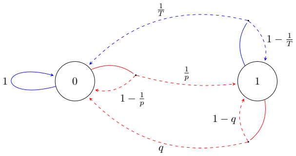
Let p = 1−ε D and q = 1 D. The set of states isS = {0, 1, . . . , S′} and the set of actions isA = {0, 1, . . . , S′}. The reward function r : S × A → [0, 1] is defined to be 1 whens ̸= 0 and a ≤ 1, and 0 otherwise. We define an index set Θ = {0, 1}S′ . For eachθ ∈ Θ, we define the transition matrixPθ as follows: s a Pθ(s′|s, a) 0 0 (1 − q)I(s′ = s) + q S...
-
[21]
At state 0, which has a reward of 0, the agent will likely be trapped for a long time before returning to one of states1, . . . , S′. See Figure 3 for a diagram of the MDP(Pθ, r) for θ = (0, . . . ,0). We now state some easily verifiable facts about the MDP(Pθ, r): • The MDP hasS states, is unichain, and has diameter1 q + 1 1/2 = D + 2 = T. • There is a u...
-
[22]
D.1 Auxiliary lemmas Lemma D.1
Thus, plugging back into Equation 52 yields max θ Pθ,n ρ∗ θ − ρA (D) θ > c3 r T S m ! ≥ 1 64 , with c3 = 2−17. D.1 Auxiliary lemmas Lemma D.1. Let π be a stationary policy on MDPMθ. Then ρπ θ ≤ 1 + ε2 2 − ε(1 − Lπ θ /S′) . Proof. A routine computation (see Lemma D.7) yields ρπ θ = q S′ PS′ s=1 1 κs 1 + q S′ PS′ s=1 1 κs , where κs = Lπ θ (s)q +(1 − Lπ θ (...
-
[23]
Lemma D.2 (Gilbert-VarshamovLemma[Massart,2007, Lemma4.7])
Consequently, ρπ θ ≤ λ 1 + λ ≤ 1 1−ε(1−Lπ θ /S′) + ε2 1 + 1 1−ε(1−Lπ θ /S′) + ε2 ≤ 1 + ε2 2 − ε(1 − Lπ θ /S′) . Lemma D.2 (Gilbert-VarshamovLemma[Massart,2007, Lemma4.7]) . Let d ≥ 8. There existsΩd ⊂ {0, 1}d such that |Ωd| ≥ 2d/8 and ∥ω − ω′∥1 ≥ d/8 for all ω ̸= ω′ ∈ Ωd. Lemma D.3. For any θ, θ′ ∈ Θ, we have KL(Pθ,n ∥ Pθ′,n) ≤ S′ 16 − 1 log 2. Proof. Let...
work page 2007
-
[24]
Incase(55), wehave Qβ(bPsa, V ′) = Qβ(bPsa, V )ontheentireinterval U andalsothatforany V ′(x) ∈ U, Qβ(bPsa, V ) > V ′(x) (since the(1−β)-percentile is achieved at some states′ ∈ S >), soTβ(bPsa, V ′)(x) = V ′(x) and Tβ(bPsa, V ′)(s′) = Tβ(bPsa, V )(s′) for all s′ ̸= x. Therefore dTβ(bPsa, V ′)(s′) dV ′(x) V ′(x)=V (x) = ( 1 s′ = x 0 otherwise and deT1(V ′...
-
[25]
In case (56), we haveQβ(bPsa, V ′) = V ′(x) on the entire intervalU. Thus Tβ(bPsa, V ′)(s′) = V ′(x) if s′ ∈ S > ∪ {x}, and Tβ(bPsa, V ′)(s′) = V ′(s′) = V (s′) for s′ ∈ S<. Thus dTβ(bPsa, V ′)(s′) dV ′(x) V ′(x)=V (x) = ( 1 s′ ∈ S > ∪ {x} 0 otherwise 54 and deT1(V ′) dV ′(x) V ′(x)=V (x) = d dV ′(x) V ′(x)=V (x) bPsaTβ(bPsa, V ′) − β Tβ(bPsa, V ′) span =...
-
[26]
Also mins′ V ′(s′) < V ′(x) on U, so mins′ V ′(s′) = mins′ V (s′) on U
In case (57), we haveQβ(bPsa, V ′) = Qβ(bPsa, V ) and also that Tβ(bPsa, V ′)(x) = Qβ(bPsa, V ) < V ′(x) (since V ′(x) < Q β(bPsa, V ) in this case), so Tβ(bPsa, V ′) = Tβ(bPsa, V ) on the interval U. Also mins′ V ′(s′) < V ′(x) on U, so mins′ V ′(s′) = mins′ V (s′) on U. Thus dTβ(bPsa, V ′)(s′) dV ′(x) V ′(x)=V (x) = 0 for all s′ ∈ S, and deT1(V ′) dV ′(...
-
[27]
And by a similar argument, g(z) < r 2 would imply z ≤ z − δ
Indeed, if we hadg(z) > r 2, then by continuity of g there would existδ > 0 such that g(t) > r 2 for t ∈ [z, z + δ], which would imply thatz ≥ z + δ. And by a similar argument, g(z) < r 2 would imply z ≤ z − δ. At z the right-derivative is nonnegative, so there existsw ∈ (z, y] such that f(t)−f(z) t−z > r 2 for allt ∈ (z, w]. Consequently, for allt ∈ (z, ...
discussion (0)
Sign in with ORCID, Apple, or X to comment. Anyone can read and Pith papers without signing in.