REVIEW 3 major objections 5 minor 38 references
Aggregating Local Saliency Maps for Semi-Global Explainable Image Classification
T0 review · 3 major / 5 minor · reviewed 2026-08-06 · deepseek-v4-flash
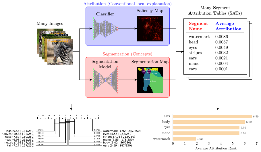
Pith's one-line read This paper introduces Segment Attribution Tables, which aggregate per-image saliency maps over named image segments to expose spurious correlations, such as reliance on watermarks, that standard accuracy metrics miss.
desk verdict Useful, cleanly described aggregation tool, but the headline 'reveal spurious correlations' overstates what the experiments show: the watermark shortcut is prompted by name, so the toy experiment is a known-feature check, not a discovery. read the letter →
The pith
A machine-rendered reading of the paper's core claim, the machinery that carries it, and where it could break.
The reading
What carries the argument
The central object is the Segment Attribution Table: for each image, the saliency map is averaged over each named segment mask, with the absolute value taken after averaging, giving $\bar{a}_i = \frac{1}{Z_i}\sum_{x,y}(M_i \odot A)_{x,y}$, and segments are ranked by this mean attribution. Aggregation across images is done two ways: relative averaging over the SATs in which a segment appears, and absolute averaging with zero-fill for absent segments. Ranking within each image before aggregation is what makes the method comparable across images and saliency methods; the named masks, produced by an open-set segmentation model prompted with a fixed label list, are what let the table speak in concepts rather than pixel coordinates.
What would settle it
Replace the saliency maps in the toy-watermark experiment with random smooth maps that respect the same segment masks; if the watermark segment's mean rank still increases with training watermark prevalence, the SAT signal is an artefact of segmentation and ranking rather than evidence of model reliance.
Extended reading notes
Core claim
SATs convert a local saliency map into a per-image ranking of named segments by mean absolute attribution, then aggregate those rankings across images to produce a semi-global table. In the toy watermark study, the mean attribution rank of the watermark segment falls from roughly 9.7 at 0% watermark prevalence to 1.92 at 50%, while clean test accuracy barely moves until past 25%; the paper reads this as evidence that SATs reveal shortcut reliance that accuracy metrics miss. The same aggregation separates a biased action-recognition model, which ranks environment segments such as rock, water, and sky above the person, from a less-biased model that reverses that ordering.
Load-bearing premise
The method only surfaces shortcuts that the analyst has named in the segmentation prompt and that the segmentation model can actually detect; a shortcut outside that set has no row in the table and remains invisible to the analysis.
Editorial extensions
If this is right
- A watermark shortcut injected into zebra images becomes the top-ranked segment at 50% training prevalence (mean attribution rank 1.92), while clean test accuracy stays close to baseline until past 25% watermarking.
- SATs work with any heatmap-based explanation, including SHAP, LIME, and attention maps, provided a segmentation map with named segments is available.
- Ranking segments within each image before aggregation makes SAT comparisons across saliency methods and models possible without explicit normalisation.
- On the BAR dataset, SATs separate a biased classifier, which ranks environment segments above the person, from a less-biased classifier that reverses that ordering.
- Aggregated SATs can be grouped or filtered by contextual metadata such as segment position and mask size, allowing targeted analysis of rare edge cases.
Reading between the lines
- The toy-watermark demonstration only works because "watermark" is one of the prompted segment labels; a shortcut that the segmentation model cannot isolate, or that the analyst does not name in advance, would not appear as a row in the table, so the paper does not yet establish discovery of truly unknown patterns.
- Because the pipeline averages raw saliency values, its outputs inherit any instability or edge-bias of the chosen saliency method; a sanity check with random attributions would show whether a rising watermark rank reflects model reliance or segmentation artefacts.
- Ranking by mean attribution suggests a natural training objective: penalise the rank of undesired segments or reward the rank of desired ones, turning SATs from a diagnostic into a debiasing method.
- Since the aggregation needs only a saliency map and a named segmentation, the same table could be applied to vision-language or generative models whenever attention maps over image regions are available.
Editorial analysis
A structured set of objections, weighed in public.
Referee Report
Summary. The paper introduces Segment Attribution Tables (SATs), a method that aggregates local saliency maps over semantically named image segments (obtained from an open-set segmentation model such as DinoX) to produce semi-global summaries of which regions a classifier relies on. The method computes per-segment mean attribution, converts to ranks, and aggregates across images using relative or absolute schemes. Three experiments are presented: (1) VGG16 on ImageNet classes (Chihuahua, Firetruck, Zebra) with six saliency methods and critical difference diagrams; (2) the BAR dataset, comparing a biased and a less-biased CNN to show that SATs rank background/environment segments above the person in the biased model; and (3) a toy watermark dataset on horse/zebra images, where the prevalence of watermarks in training is varied and the watermark segment's mean attribution rank is tracked against clean and watermarked test accuracy. The central claim is that SATs reveal spurious correlations, such as reliance on backgrounds or watermarks, even when out-of-distribution accuracy changes little.
Significance. The proposed SATs are a simple, model-agnostic, and saliency-agnostic summary tool that could be practically useful for auditing classifiers. The paper includes a useful comparison of six saliency methods on a common task, and the BAR experiment demonstrates how the method can expose environment biases without an OOD test set. The watermark toy experiment is a well-designed controlled study of shortcut prevalence, and the observation that attribution rank changes earlier than accuracy is interesting. However, the headline claim that SATs can 'reveal' unknown spurious correlations is not fully supported: the watermark is explicitly added to the segmentation prompt, and the detection threshold is chosen post hoc. These issues weaken the empirical support for the discovery-oriented interpretation of the method, though the method still works as a tool for measuring reliance on pre-specified candidate segments.
major comments (3)
- [Toy Watermark Dataset] The shortcut is included in the segmentation prompt by construction: the authors state that they 'choose the same 12 labels as in the ImageNet experiment, but replace the least impactful segment (neck) with watermark.' This means the experiment measures a pre-specified region, not an unknown shortcut. The related-work section criticizes Global Saliency because 'it cannot identify previously unknown influential patterns, relying entirely on prior knowledge of the segment to be analysed'; SATs inherit the same dependence. To support the abstract's claim that SATs 'reveal spurious correlations,' the authors should add an experiment where the shortcut is not explicitly prompted, for example by using unprompted DinoX segmentation or a segment list that does not contain 'watermark,' and show that the watermark pattern can still be surfaced by the segmentation model.
- [Toy Watermark Dataset, Figure 5] The claim that 'a clear signal emerging from around 15% watermarking' is based on visual inspection of the plot, with no statistical criterion, confidence intervals, or predefined detection threshold. At 15% watermarking the watermark segment's mean rank (4.98) is close to several other segments (e.g., mane at 6.07, body at 6.50), so the 'clear signal' is not quantified. Please provide error bars (e.g., bootstrap over images) or a statistical comparison (e.g., permutation test against a non-shortcut segment) to substantiate the claim that SATs detect the shortcut earlier than the accuracy drop.
- [Understanding Model Behaviour / Results] The ImageNet experiment uses only 100 images per class and segment lists generated by ChatGPT with manual editing. The paper acknowledges this in the conclusion, but the potential selection bias in the segment lists is not analyzed. Since the segment list directly determines which segments can ever appear in a SAT, a sensitivity analysis (e.g., different prompt phrasings or segment lists) would help establish how robust the reported rankings are to the choice of segments.
minor comments (5)
- [Figure 2] The figure title contains typos: 'Watermaked' should be 'Watermarked' and 'Salinecy' should be 'Saliency'.
- [Understanding Model Behaviour] The text says 'using tensorflows pre-trained weights'; this should be 'TensorFlow's pre-trained weights'.
- [Figure 5] The y-axis label 'Mean Average Attribution Rank' is ambiguous. Clarify that it is the mean over test images of the watermark segment's rank (not an average of averages).
- [Producing SATs] The definition allows pixels to appear in multiple segment masks, but the experiments use DinoX, which likely produces non-overlapping masks. Please state explicitly whether the masks used in the experiments are disjoint.
- [Conclusion and Future Work] The paper compares six saliency methods on the Chihuahua class but does not mention how one might aggregate them; since the conclusion suggests aggregating multiple explanation methods as future work, a brief comment on the observed agreement (or lack thereof) across the six methods would be useful.
Circularity Check
No significant circularity: SATs are a definitional summary of saliency, and the watermark experiment measures a pre-specified segment rather than deriving an equivalent quantity.
full rationale
The paper contains no circular derivation. SATs are defined as a summary statistic: mean saliency per named segment, converted to a local rank, with no fitted parameters and no quantity predicted from the method's own outputs. The toy watermark experiment measures the mean attribution rank of the 'watermark' segment on a held-out watermarked test set for models trained at different watermark prevalences; this is a direct measurement, not a construction that forces the result. The paper does pre-specify the shortcut by prompting DinoX with the label 'watermark': 'Once more we segment the images using DinoX, and choose the same 12 labels as in the ImageNet experiment, but replace the least impactful segment (neck) with watermark.' This means the experiment demonstrates detection of a known artefact rather than discovery of an unknown one, which is a scope limitation and is even acknowledged by the authors in the conclusion: 'the suitability of SATs depends significantly on the segmentation maps used. Issues such as incorrect labels, undetected objects, or inappropriate granularity (e.g., identifying a whole object rather than its parts) can reduce effectiveness. While targeted prompting with open-set models mitigates some of these problems, this method requires expert oversight.' That dependence is a practical constraint, not circularity. The only self-citations are to the authors' earlier CoF tables as related work (e.g., 'CoF tables (Hinns and Martens 2024)'), and neither the SAT definition nor any experimental result relies on CoF or on an imported uniqueness theorem. External components such as DinoX, LRP, iNNvestigate, ImageNet, and BAR supply the inputs; no equation reduces to its own output.
Assumptions & free parameters
free parameters (4)
- number of prompted segments per class =
12
- mask padding width =
2 pixels
- segment name list per class =
e.g., eyes, nose, ears, head, body, legs, tail; in watermark experiment 'watermark' added and 'neck' removed
- shortcut detection threshold =
15% watermark prevalence
assumptions (3)
- domain assumption Saliency maps reliably indicate which pixels or regions drive the model prediction
- domain assumption The segmentation model (DinoX) with the given prompts produces semantically correct and consistent segments across images
- domain assumption Averaging absolute mean saliency per segment and ranking segments preserves meaningful comparisons across images
Cite this review
Pith. "Pith review of Aggregating Local Saliency Maps for Semi-Global Explainable Image Classification." pith.science (2026). https://pith.science/paper/WMK76ISP
@misc{pith2026250623247,
  author       = {Pith},
  title        = {Pith review of: Aggregating Local Saliency Maps for Semi-Global Explainable Image Classification},
  year         = {2026},
  howpublished = {\url{https://pith.science/paper/WMK76ISP}},
  note         = {Machine review of arXiv:2506.23247}
}
read the original abstract
Deep learning dominates image classification tasks, yet understanding how models arrive at predictions remains a challenge. Much research focuses on local explanations of individual predictions, such as saliency maps, which visualise the influence of specific pixels on a model's prediction. However, reviewing many of these explanations to identify recurring patterns is infeasible, while global methods often oversimplify and miss important local behaviours. To address this, we propose Segment Attribution Tables (SATs), a method for summarising local saliency explanations into (semi-)global insights. SATs take image segments (such as "eyes" in Chihuahuas) and leverage saliency maps to quantify their influence. These segments highlight concepts the model relies on across instances and reveal spurious correlations, such as reliance on backgrounds or watermarks, even when out-of-distribution test performance sees little change. SATs can explain any classifier for which a form of saliency map can be produced, using segmentation maps that provide named segments. SATs bridge the gap between oversimplified global summaries and overly detailed local explanations, offering a practical tool for analysing and debugging image classifiers.
Figures


Figures from the paper (4 more)


Reference graph
Works this paper leans on
-
[1]
, " * write output.state after.block = add.period write newline
ENTRY address archivePrefix author booktitle chapter edition editor eid eprint howpublished institution isbn journal key month note number organization pages publisher school series title type volume year label extra.label sort.label short.list INTEGERS output.state before.all mid.sentence after.sentence after.block FUNCTION init.state.consts #0 'before.a...
-
[2]
write newline
" write newline "" before.all 'output.state := FUNCTION n.dashify 't := "" t empty not t #1 #1 substring "-" = t #1 #2 substring "--" = not "--" * t #2 global.max substring 't := t #1 #1 substring "-" = "-" * t #2 global.max substring 't := while if t #1 #1 substring * t #2 global.max substring 't := if while FUNCTION word.in bbl.in capitalize " " * FUNCT...
-
[3]
Alber, M.; Lapuschkin, S.; Seegerer, P.; H \"a gele, M.; Sch \"u tt, K. T.; Montavon, G.; Samek, W.; M \"u ller, K.-R.; D \"a hne, S.; and Kindermans, P.-J. 2019. iNNvestigate Neural Networks! Journal of Machine Learning Research, 20(93): 1--8
work page 2019
-
[4]
Alom, M. Z.; Taha, T. M.; Yakopcic, C.; Westberg, S.; Sidike, P.; Nasrin, M. S.; Van Esesn, B. C.; Awwal, A. A. S.; and Asari, V. K. 2018. The history began from alexnet: A comprehensive survey on deep learning approaches. arXiv preprint arXiv:1803.01164
arXiv 2018
-
[5]
Bach, S.; Binder, A.; Montavon, G.; Klauschen, F.; M \"u ller, K.-R.; and Samek, W. 2015. On pixel-wise explanations for non-linear classifier decisions by layer-wise relevance propagation. PloS one, 10(7): e0130140
work page 2015
-
[6]
Chen, L.; Li, S.; Bai, Q.; Yang, J.; Jiang, S.; and Miao, Y. 2021. Review of image classification algorithms based on convolutional neural networks. Remote Sensing, 13(22): 4712
work page 2021
-
[7]
DeGrave, A. J.; Janizek, J. D.; and Lee, S.-I. 2021. AI for radiographic COVID-19 detection selects shortcuts over signal. Nature Machine Intelligence, 3(7): 610--619
work page 2021
-
[8]
Geirhos, R.; Jacobsen, J.-H.; Michaelis, C.; Zemel, R.; Brendel, W.; Bethge, M.; and Wichmann, F. A. 2020. Shortcut learning in deep neural networks. Nature Machine Intelligence, 2(11): 665--673
work page 2020
Show all 38 references
-
[9]
Y.; and Kim, B
Ghorbani, A.; Wexler, J.; Zou, J. Y.; and Kim, B. 2019. Towards automatic concept-based explanations. Advances in neural information processing systems, 32
2019
-
[10]
Hinns, J.; and Martens, D. 2024. Exposing image classifier shortcuts with counterfactual frequency (cof) tables. arXiv preprint arXiv:2405.15661
2024 arXiv
-
[11]
Kim, B.; Wattenberg, M.; Gilmer, J.; Cai, C.; Wexler, J.; Viegas, F.; et al. 2018. Interpretability beyond feature attribution: Quantitative testing with concept activation vectors (tcav). In International conference on machine learning, 2668--2677. PMLR
2018
-
[12]
W.; Nguyen, T.; Tang, Y
Koh, P. W.; Nguyen, T.; Tang, Y. S.; Mussmann, S.; Pierson, E.; Kim, B.; and Liang, P. 2020. Concept bottleneck models. In International conference on machine learning, 5338--5348. PMLR
2020
-
[13]
a ldchen, S.; Binder, A.; Montavon, G.; Samek, W.; and M \
Lapuschkin, S.; W \"a ldchen, S.; Binder, A.; Montavon, G.; Samek, W.; and M \"u ller, K.-R. 2019. Unmasking Clever Hans predictors and assessing what machines really learn. Nature communications, 10(1): 1096
2019
-
[14]
J.; Srinivas, S.; Bhalla, U.; and Lakkaraju, H
Li, A. J.; Srinivas, S.; Bhalla, U.; and Lakkaraju, H. 2025. Interpretability Illusions with Sparse Autoencoders: Evaluating Robustness of Concept Representations. arXiv preprint arXiv:2505.16004
2025
-
[15]
M.; and Lee, S.-I
Lundberg, S. M.; and Lee, S.-I. 2017. A unified approach to interpreting model predictions. Advances in neural information processing systems, 30
2017
-
[16]
Middlehurst, M.; Ismail-Fawaz, A.; Guillaume, A.; Holder, C.; Guijo-Rubio, D.; Bulatova, G.; Tsaprounis, L.; Mentel, L.; Walter, M.; Sch \"a fer, P.; and Bagnall, A. 2024. aeon: a Python Toolkit for Learning from Time Series. Journal of Machine Learning Research, 25(289): 1--10
2024
-
[17]
Molnar, C. 2025. Interpretable Machine Learning. 3 edition. ISBN 978-3-911578-03-5
2025
-
[18]
Montavon, G.; Lapuschkin, S.; Binder, A.; Samek, W.; and M \"u ller, K.-R. 2017. Explaining nonlinear classification decisions with deep taylor decomposition. Pattern recognition, 65: 211--222
2017
-
[19]
Nam, J.; Cha, H.; Ahn, S.; Lee, J.; and Shin, J. 2020. Learning from Failure: Training Debiased Classifier from Biased Classifier. In Advances in Neural Information Processing Systems
2020
-
[20]
G.; Athalye, A.; and Mueller, J
Northcutt, C. G.; Athalye, A.; and Mueller, J. 2021. Pervasive Label Errors in Test Sets Destabilize Machine Learning Benchmarks. In Proceedings of the 35th Conference on Neural Information Processing Systems Track on Datasets and Benchmarks
2021
-
[21]
T.; Wei, M
Pfau, J.; Young, A. T.; Wei, M. L.; and Keiser, M. J. 2019. Global saliency: aggregating saliency maps to assess dataset artefact bias. arXiv preprint arXiv:1910.07604
2019 arXiv
-
[22]
Ren, T.; Chen, Y.; Jiang, Q.; Zeng, Z.; Xiong, Y.; Liu, W.; Ma, Z.; Shen, J.; Gao, Y.; Jiang, X.; Chen, X.; Song, Z.; Zhang, Y.; Huang, H.; Gao, H.; Liu, S.; Zhang, H.; Li, F.; Yu, K.; and Zhang, L. 2024 a . DINO-X: A Unified Vision Model for Open-World Object Detection and Un...
2024 arXiv
-
[23]
Ren, T.; Liu, S.; Zeng, A.; Lin, J.; Li, K.; Cao, H.; Chen, J.; Huang, X.; Chen, Y.; Yan, F.; et al. 2024 b . Grounded sam: Assembling open-world models for diverse visual tasks. arXiv preprint arXiv:2401.14159
2024 arXiv
-
[24]
Why should i trust you?
Ribeiro, M. T.; Singh, S.; and Guestrin, C. 2016. " Why should i trust you?" Explaining the predictions of any classifier. In Proceedings of the 22nd ACM SIGKDD international conference on knowledge discovery and data mining, 1135--1144
2016
-
[25]
Rieger, L.; and Hansen, L. K. 2019. Aggregating explanation methods for stable and robust explainability. arXiv preprint arXiv:1903.00519
2019 arXiv
-
[26]
Russakovsky, O.; Deng, J.; Su, H.; Krause, J.; Satheesh, S.; Ma, S.; Huang, Z.; Karpathy, A.; Khosla, A.; Bernstein, M.; et al. 2015. Imagenet large scale visual recognition challenge. International journal of computer vision, 115: 211--252
2015
-
[27]
Samek, W.; and M \"u ller, K.-R. 2019. Towards explainable artificial intelligence. In Explainable AI: interpreting, explaining and visualizing deep learning, 5--22. Springer
2019
-
[28]
R.; Cogswell, M.; Das, A.; Vedantam, R.; Parikh, D.; and Batra, D
Selvaraju, R. R.; Cogswell, M.; Das, A.; Vedantam, R.; Parikh, D.; and Batra, D. 2017. Grad-cam: Visual explanations from deep networks via gradient-based localization. In Proceedings of the IEEE international conference on computer vision, 618--626
2017
-
[29]
Simonyan, K.; and Zisserman, A. 2014. Very deep convolutional networks for large-scale image recognition. arXiv preprint arXiv:1409.1556
2014 arXiv
-
[30]
Smilkov, D.; Thorat, N.; Kim, B.; Vi \'e gas, F.; and Wattenberg, M. 2017. Smoothgrad: removing noise by adding noise. arXiv preprint arXiv:1706.03825
2017 arXiv
-
[31]
Sun, A.; Ma, P.; Yuan, Y.; and Wang, S. 2023. Explain any concept: Segment anything meets concept-based explanation. Advances in Neural Information Processing Systems, 36: 21826--21840
2023
-
[32]
Sundararajan, M.; Taly, A.; and Yan, Q. 2017. Axiomatic attribution for deep networks. In International conference on machine learning, 3319--3328. PMLR
2017
-
[33]
Van Der Linden, I.; Haned, H.; and Kanoulas, E. 2019. Global aggregations of local explanations for black box models. arXiv preprint arXiv:1907.03039
2019 arXiv
-
[34]
K.; Fink, C.; Toberer, F.; Enk, A.; Deinlein, T.; Hofmann-Wellenhof, R.; Thomas, L.; Lallas, A.; Blum, A.; Stolz, W.; et al
Winkler, J. K.; Fink, C.; Toberer, F.; Enk, A.; Deinlein, T.; Hofmann-Wellenhof, R.; Thomas, L.; Lallas, A.; Blum, A.; Stolz, W.; et al. 2019. Association between surgical skin markings in dermoscopic images and diagnostic performance of a deep learning convolutional neural ne...
2019
-
[35]
Yeh, C.-K.; Kim, B.; Arik, S.; Li, C.-L.; Pfister, T.; and Ravikumar, P. 2020. On completeness-aware concept-based explanations in deep neural networks. Advances in neural information processing systems, 33: 20554--20565
2020
-
[36]
Yuksekgonul, M.; Wang, M.; and Zou, J. 2022. Post-hoc concept bottleneck models. arXiv preprint arXiv:2205.15480
2022 arXiv
-
[37]
R.; Badgeley, M
Zech, J. R.; Badgeley, M. A.; Liu, M.; Costa, A. B.; Titano, J. J.; and Oermann, E. K. 2018. Variable generalization performance of a deep learning model to detect pneumonia in chest radiographs: a cross-sectional study. PLoS medicine, 15(11): e1002683
2018
-
[38]
T.; and Hermanns, H
Zhang, H.; Figueroa, F. T.; and Hermanns, H. 2024. Saliency Maps Give a False Sense of Explanability to Image Classifiers: An Empirical Evaluation across Methods and Metrics. In The 16th Asian Conference on Machine Learning (Conference Track)
2024
Reviewed August 6, 2026 · model on record in the stance chip above.
Discussion (0). Continue with ORCID to comment.