REVIEW 4 major objections 6 minor 37 references
Sample Margin-Aware Recalibration of Temperature Scaling
T0 review · 4 major / 6 minor · reviewed 2026-08-06 · deepseek-v4-flash
Pith's one-line read A 49-parameter calibrator keys off the top-two logit gap to beat temperature scaling.
desk verdict A useful empirical calibration method with a broken proof; the logit-gap idea stands on its own, but the theory section needs a fix. read the letter →
The pith
A machine-rendered reading of the paper's core claim, the machinery that carries it, and where it could break.
The reading
What carries the argument
The load-bearing object is the logit gap $g_i = z_{i,\max} - z_{i,2\mathrm{nd}}$, a scalar derived from the top two logits, combined with the scalar-to-scalar regression $T = h_\phi(g_i)$ implemented as a one-hidden-layer MLP with a $\mathrm{softplus}$ output. A second component is the SoftECE objective, which replaces hard bin membership with soft weights $w_{i,b} \propto \exp(-\alpha(\hat p_i - c_b)^2)$; as $\alpha \to 0$ it becomes global accuracy and as bin width shrinks it approaches pointwise accuracy, so $\alpha$ and bin count act as explicit bias-variance knobs. The theoretical carrier is Proposition 3.2, which bounds the temperature $T$ in terms of $g$, the target confidence $\hat p$, and the class count $K$, justifying the use of $g$ as a control signal for recalibration.
What would settle it
Take a validation set and, for each sample, compute the oracle temperature that best recalibrates that sample by grid search. Split samples into groups with equal logit gap $g$ but different values of the sum of the remaining logits. If, within a fixed-$g$ group, the oracle temperature varies substantially across subgroups and a method that additionally uses the sum or $z_{\max}$ achieves lower ECE than SMART, then $g$ alone is not sufficient and the central claim fails.
Extended reading notes
Core claim
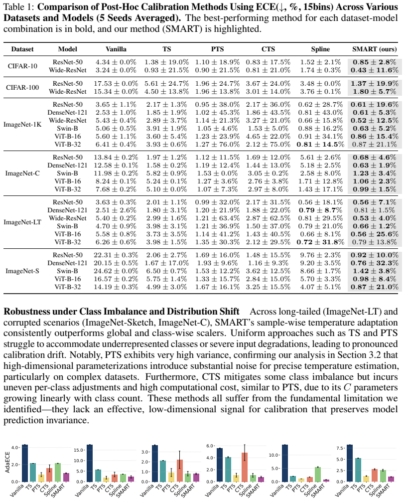
On the paper's own terms, the central discovery is that the margin between the largest and second-largest logit, $g_i = z_{i,\max} - z_{i,2\mathrm{nd}}$, is the right scalar input for sample-wise temperature scaling. The authors prove that the implicit temperature $T$ that moves the softmax probability to a target confidence $\hat p$ is unbounded when only $z_{\max}$ is fixed (Proposition 3.1), but is sandwiched by $g$: $-g/\log(S) < T \le -g/\log(S/(K-1))$, where $S = 1/\hat p - 1$ (Proposition 3.2). A one-hidden-layer network $T = h_\phi(g_i)$ trained with the soft-binned SoftECE objective then achieves the lowest ECE and AdaECE in nearly all reported comparisons, with 49 parameters, exact accuracy preservation, and stable behavior down to 50 validation samples, including on ImageNet corruption, long-tailed, and sketch variants.
Load-bearing premise
The method collapses if the gap between the top two logits does not carry enough information to determine the right temperature change, because the network never sees the rest of the logit vector.
Editorial extensions
If this is right
- A calibrator whose parameter count does not grow with the number of classes is enough for large-scale tasks: 49 parameters serve ImageNet's 1,000 classes, whereas class-wise and spline calibrators scale linearly with class count.
- Data-efficient recalibration becomes practical: the method reports stable calibration error with validation sets around 50 samples, a regime where full-logit parametric methods show high variance.
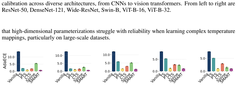
- Calibration under distribution shift is attainable with a scalar margin signal: SMART stays stable on corrupted, long-tailed, and sketch inputs where spline calibration degrades sharply.
- Accuracy is preserved by construction while confidence is repaired, because temperature scaling does not change the argmax; the reported tables confirm zero accuracy loss across all combinations.
- SMART composes with training-time calibration losses: applying it on top of Brier, MMCE, label smoothing, or focal-loss training reduces ECE and AdaECE in nearly all table entries.
Reading between the lines
- If the logit gap is as informative as claimed, the same scalar could be reused outside calibration, for example as a feature for selective prediction or out-of-distribution detection, since it already encodes decision-boundary proximity.
- The paper's bound is an interval, not an equality, so the residual information in the other logits is not proven irrelevant; conditioning the temperature map on $z_{\max}$ or the sum of the remaining logits may push ECE lower than the reported 49-parameter version.
- The appendix's finding that high-gap samples are under-confident suggests SMART is effectively learning a margin-to-confidence correction; if that correction is largely architecture-independent, the same learned map might transfer across models without retraining.
- Because SoftECE's weighting parameter $\alpha$ and bin count are the explicit bias-variance knobs, adapting them to the validation-set size could extend the data-efficiency results beyond the fixed settings reported.
Editorial analysis
A structured set of objections, weighed in public.
Referee Report
Summary. The paper proposes SMART, a post-hoc calibration method that predicts a per-sample temperature from the gap between the top-two logits. A small MLP maps the normalized gap to a positive temperature, and the model is trained by minimizing a soft-binned ECE loss on validation logits. The authors claim that SMART achieves state-of-the-art calibration on CIFAR-10/100, ImageNet-1K, and corrupted, long-tailed, and sketch-shifted variants, while using only 49 parameters and as few as 50 calibration samples. Theoretical support is offered by Propositions 3.1 and 3.2, which aim to show that the optimal temperature for reaching a target confidence is tightly bounded by the logit gap. The paper also reports ablations on the input signal, loss function, validation size, bin count, runtime, and additional metrics such as AdaECE and CECE.
Significance. The logit-gap design is a genuinely simple and appealing idea: it is scalar, prediction-preserving, and cheap, and the soft-bin objective is well matched to small validation sets. The empirical study is broad, covering multiple architectures, several distribution-shift scenarios, multiple metrics, seed-averaged results, and ablation tables. If the main-table rankings survive standard-size validation sets, this would be a practically useful method. However, the theoretical contribution does not establish that the gap is a sufficient statistic for optimal temperatures, and the headline claim of consistent superiority is contradicted by several Spline entries in Table 1. Credit is due for reporting parameter counts, runtime, bin sensitivity, and validation-size curves, which help the reader judge the method's trade-offs.
major comments (4)
- [§3.4, Eq. (19)] Proposition 3.2 does not establish sufficiency of g for T. The interval in Eq. (19) is -g/log S < T <= -g/log(S/(K-1)) with S = sum_{j != M} exp((z_j - z_M)/T), so the endpoints depend on the full logit vector and on T itself; two samples with the same gap can require very different temperatures. The paper should either prove a bound in terms of g alone, quantify the residual dependence on the remaining logits, or explicitly present the result as an empirical motivation rather than a theoretical foundation.
- [Table 1 and §4.2] The statement that SMART 'consistently outperforms' the baselines is not supported by Table 1: Spline beats SMART on ImageNet-1K ViT-B-32 (0.81 vs 0.87), on ImageNet-LT ViT-B-32 (0.72 vs 0.79), and on ImageNet-LT DenseNet-121 (0.79 vs 0.81). The abstract and Section 4.2 need qualification, and these counterexamples should be analyzed, for example by checking whether they correspond to particular gap regimes or class counts.
- [§4.1, Table 1] The main ImageNet comparisons use a 50-sample validation set, which is 0.1% of the original 50,000-sample validation split. This protocol strongly favors the 49-parameter SMART over PTS, CTS, and Spline, whose parameter counts grow with the number of classes. The paper should add at least one main-table comparison with a conventional validation size, such as 2,000 or 5,000 samples, and should report how baseline hyperparameters were selected under the 50-sample budget. Until then, the SOTA claim is mostly a claim about the ultra-low-data regime.
- [§3.3–3.4, Eq. (10) and Eq. (11)] The theoretical analysis solves a per-sample equation with a fixed target confidence p-hat, while the training objective SoftECE in Eq. (10) is a binned, sample-weighted average over all samples and bins. The paper does not show that a temperature satisfying Eq. (11) minimizes Eq. (10), nor how the target p-hat is derived during training. This is a missing link between the proof and the actual objective; at minimum, the theory section should be labeled as motivation.
minor comments (6)
- [Eq. (19)] Equation (19) uses n-1 while the class count is K elsewhere; the notation should be unified.
- [§3.3] Section 3.3 uses b both as a bin index and as a bin width in the phrase 'setting b -> 0', which makes the limiting statement confusing.
- [§4.1 and Fig. 4] Section 4.1 says the validation set is '0.001' of the original validation set, but Figure 4 labels the axis '0.001%'; since 50 samples is 0.1% of 50,000, the text and the figure should be reconciled.
- [Table 6] In Table 6, the Spline accuracy for DenseNet-121 on ImageNet-C is 40.83%, identical to the Swin-B value and 19.6 points above the Vanilla baseline; this looks like a copy error and should be checked.
- [Fig. 2] Figure 2's axis labels appear as raw Unicode glyphs in the submitted PDF; these need to be regenerated for readability.
- [References [4] and [36]] References [4] and [36] both list a 'Frenkel' author, but the two entries appear to be different papers; the citations in Sections 2 and 4.2 should be checked for consistency.
Circularity Check
No significant circularity: SMART's temperature mapping is a standard supervised validation fit, and the theoretical logit-gap bound is derived algebraically from the softmax equation without using the fitted parameters.
full rationale
SMART's derivation chain is self-contained. The temperature network in Eq. (6) is trained on a validation split by minimizing the SoftECE objective in Eq. (10); this is a standard supervised fit, not a construction that builds the test answer into the predictor. The theoretical bound in Props. 3.1 and 3.2 is obtained by manipulating the softmax equation (11): substituting the ordering inequality (17) into the sum identity (18) yields the interval in Eq. (19), and none of those steps substitutes h_phi or uses fitted weights. The SOTA claim is checked against external baselines (TS, PTS, CTS, Spline) on held-out test sets in Tables 1, 3, and 7, so the empirical comparison is not forced by construction. The skeptic's concern that the logit gap is not shown to be a sufficient statistic for the optimal temperature is a correctness or completeness issue about the strength of the theory, not circularity: an incomplete justification does not make the method's output equivalent to its input by definition. SoftECE is adopted from prior external work [8], and the only same-author reference [17] is not cited in the body and plays no load-bearing role. No circular step, fitted-parameter-as-prediction reduction, or self-citation dependency is present.
Assumptions & free parameters
free parameters (6)
- MLP weights and biases (W1, W2, b1, b2) =
49 parameters at d=16 (3d+1)
- Logit-gap normalization statistics (mu_g, sigma_g) =
Not reported numerically
- SoftECE smoothing coefficient alpha =
Not reported
- Number of bins B in SoftECE =
15 in reported ECE/AdaECE tables
- Hidden dimension d =
16 (also d=1, d=2 in Fig. 1a)
- MLP training hyperparameters (epochs, learning rate, optimizer) =
Not reported
assumptions (5)
- domain assumption The per-sample temperature mapping T = h_phi(g) with a scalar input can represent the optimal temperature adjustment well enough to improve calibration.
- domain assumption The validation set is representative of the test distribution, so minimizing SoftECE on validation samples transfers to test calibration.
- standard math The strict inequality e^{-g/T} < S in Eq. (18) holds.
- domain assumption The theoretical analysis assumes a per-sample target confidence \hat p that is determined by minimizing the SoftECE objective (Eq. 11).
- domain assumption The logit gap is a robust, denoised signal that captures decision-boundary uncertainty better than entropy, confidence, or full logits.
Cite this review
Pith. "Pith review of Sample Margin-Aware Recalibration of Temperature Scaling." pith.science (2026). https://pith.science/paper/IOOTMKL7
@misc{pith2026250623492,
  author       = {Pith},
  title        = {Pith review of: Sample Margin-Aware Recalibration of Temperature Scaling},
  year         = {2026},
  howpublished = {\url{https://pith.science/paper/IOOTMKL7}},
  note         = {Machine review of arXiv:2506.23492}
}
read the original abstract
Recent advances in deep learning have significantly improved predictive accuracy. However, modern neural networks remain systematically overconfident, posing risks for deployment in safety-critical scenarios. Current post-hoc calibration methods face a fundamental dilemma: global approaches like Temperature Scaling apply uniform adjustments across all samples, introducing high bias despite computational efficiency, while more expressive methods that operate on full logit distributions suffer from high variance due to noisy high-dimensional inputs and insufficient validation data. To address these challenges, we propose Sample Margin-Aware Recalibration of Temperature (SMART), a lightweight, data-efficient recalibration method that precisely scales logits based on the margin between the top two logits -- termed the logit gap. Specifically, the logit gap serves as a denoised, scalar signal directly tied to decision boundary uncertainty, providing a robust indicator that avoids the noise inherent in high-dimensional logit spaces while preserving model prediction invariance. Meanwhile, SMART employs a novel soft-binned Expected Calibration Error (SoftECE) objective that balances model bias and variance through adaptive binning, enabling stable parameter updates even with extremely limited calibration data. Extensive evaluations across diverse datasets and architectures demonstrate that SMART achieves state-of-the-art calibration performance even with substantially fewer parameters compared to existing parametric methods, offering a principled, robust, and highly efficient solution for practical uncertainty quantification in neural network predictions. The source code is available at: https://anonymous.4open.science/r/SMART-8B11.
Figures


Figures from the paper (11 more)




Reference graph
Works this paper leans on
-
[1]
On calibration of modern neural networks
Chuan Guo, Geoff Pleiss, Yu Sun, and Kilian Q Weinberger. On calibration of modern neural networks. In Proceedings of the 34th International Conference on Machine Learning (ICML), pages 1321–1330. PMLR, 2017
work page 2017
-
[2]
Obtaining well calibrated probabilities using bayesian binning
Mahdi Pakdaman Naeini, Gregory Cooper, and Milos Hauskrecht. Obtaining well calibrated probabilities using bayesian binning. Proceedings of the Twenty-Ninth AAAI Conference on Artificial Intelligence, 2015
work page 2015
-
[3]
Obtaining calibrated probability estimates from decision trees and naive bayesian classifiers
Bianca Zadrozny and Charles Elkan. Obtaining calibrated probability estimates from decision trees and naive bayesian classifiers. In Proceedings of the Eighteenth International Conference on Machine Learning, pages 609–616. Morgan Kaufmann Publishers Inc., 2001
work page 2001
-
[4]
Network calibration using differentiable classification performance metrics
Yoni Frenkel, Arseny Potapov, and Sivan Avidar. Network calibration using differentiable classification performance metrics. In ICASSP 2021-2021 IEEE International Conference on Acoustics, Speech and Signal Processing, pages 3220–3224. IEEE, 2021
work page 2021
-
[5]
Meelis Kull, Miquel Perello Nieto, Markus Kängsepp, Telmo Silva Filho, Hao Song, and Peter Flach. Beyond temperature scaling: Obtaining well-calibrated multi-class probabilities with dirichlet calibration. In Advances in Neural Information Processing Systems , pages 12316–12326, 2019
work page 2019
-
[6]
Christian Tomani, Daniel Cremers, and Florian Buettner. Parameterized temperature scaling for boosting the expressive power in post-hoc uncertainty calibration. In Computer Vision – ECCV 2022, volume 13673 of Lecture Notes in Computer Science, pages 555–569. Springer, 2022
work page 2022
-
[7]
Trainable calibration measures for neural networks from kernel mean embeddings
Aviral Kumar, Sunita Sarawagi, and Ujjwal Jain. Trainable calibration measures for neural networks from kernel mean embeddings. In International Conference on Machine Learning, pages 2805–2814. PMLR, 2018
work page 2018
-
[8]
Soft calibration objectives for neural networks
Archit Karandikar, Nicholas Cain, Dustin Tran, Balaji Lakshminarayanan, Jonathon Shlens, Michael C Mozer, and Becca Roelofs. Soft calibration objectives for neural networks. Advances in Neural Information Processing Systems, 34:29768–29779, 2021
work page 2021
Show all 37 references
-
[9]
Obtaining well calibrated probabilities using bayesian binning
Mahdi Pakdaman Naeini, Gregory Cooper, and Milos Hauskrecht. Obtaining well calibrated probabilities using bayesian binning. In Proceedings of the AAAI Conference on Artificial Intelligence, volume 29, 2015
2015
-
[10]
Calibration of neural networks using splines
Kartik Gupta, Amir Rahimi, Thalaiyasingam Ajanthan, Thomas Mensink, Cristian Sminchis- escu, and Richard Hartley. Calibration of neural networks using splines. In International Conference on Learning Representations, 2021
2021
-
[11]
Beyond global calibration: Group calibration via multiple comparison errors
Lu Yang, Kai Zhang, Qing Wang, Sanvesh Zhang, and Caroline Uhler. Beyond global calibration: Group calibration via multiple comparison errors. arXiv preprint arXiv:2401.15798, 2024
2024 arXiv
-
[12]
Proximity-informed calibration for deep neural networks
Miao Xiong, Ailin Deng, Pang Wei Koh, Jiaying Wu, Shen Li, Jianqing Xu, and Bryan Hooi. Proximity-informed calibration for deep neural networks. In Thirty-seventh Conference on Neural Information Processing Systems, 2023
2023
-
[13]
Multicalibration: Calibration for the (computationally-identifiable) masses
Ursula Hebert-Johnson, Michael Kim, Omer Reingold, and Guy Rothblum. Multicalibration: Calibration for the (computationally-identifiable) masses. Proceedings of the 35th International Conference on Machine Learning, 2018
2018
-
[14]
Verification of forecasts expressed in terms of probability
Glenn W Brier. Verification of forecasts expressed in terms of probability. Monthly Weather Review, 78(1):1–3, 1950
1950
-
[15]
Re- thinking the inception architecture for computer vision
Christian Szegedy, Vincent Vanhoucke, Sergey Ioffe, Jon Shlens, and Zbigniew Wojna. Re- thinking the inception architecture for computer vision. In Proceedings of the IEEE Conference on Computer Vision and Pattern Recognition, pages 2818–2826, 2016
2016
-
[16]
Calibrating deep neural networks using focal loss
Jishnu Mukhoti, Viveka Kulharia, Amartya Sanyal, Stuart Golodetz, Philip Torr, and Puneet Dokania. Calibrating deep neural networks using focal loss. In Advances in Neural Information Processing Systems, pages 15744–15755, 2020. 11
2020
-
[17]
Dual focal loss for calibration
Linxi Tao, Mingming Dong, and Chang Xu. Dual focal loss for calibration. In Proceedings of the 40th International Conference on Machine Learning (ICML). PMLR, 2023
2023
-
[18]
Simple and scalable predictive uncertainty estimation using deep ensembles
Balaji Lakshminarayanan, Alexander Pritzel, and Charles Blundell. Simple and scalable predictive uncertainty estimation using deep ensembles. In Advances in Neural Information Processing Systems, pages 6402–6413, 2017
2017
-
[19]
Dropout as a bayesian approximation: Representing model uncertainty in deep learning
Yarin Gal and Zoubin Ghahramani. Dropout as a bayesian approximation: Representing model uncertainty in deep learning. In International Conference on Machine Learning, pages 1050–1059, 2016
2016
-
[20]
Approaching the limit of accuracy: Residual uncertainty via test-time data augmentation
Marcel Conde, Danny Niebling, Nicolas Schilling, and Bernhard Sick. Approaching the limit of accuracy: Residual uncertainty via test-time data augmentation. In 2023 IEEE International Conference on Data Mining, pages 933–938. IEEE, 2023
2023
-
[21]
Yong-Jin Han
Jize Zhang, Bhavya Kailkhura, and T. Yong-Jin Han. Mix-n-match: Ensemble and compositional methods for uncertainty calibration in deep learning. In International Conference on Machine Learning, pages 11117–11128. PMLR, 2020
2020
-
[22]
Intra order-preserving functions for calibration of multi-class neural networks
Amir Rahimi, Amirreza Shaban, Ching-An Cheng, Byron Boots, and Richard Hartley. Intra order-preserving functions for calibration of multi-class neural networks. In Advances in Neural Information Processing Systems, pages 15829–15839, 2020
2020
-
[23]
Optimizing calibration by gaining aware of prediction correctness
Yuchi Liu, Lei Wang, Yuli Zou, James Zou, and Liang Zheng. Optimizing calibration by gaining aware of prediction correctness. arXiv preprint arXiv:2404.13016, 2024
2024 arXiv
-
[24]
Learning multiple layers of features from tiny images
Alex Krizhevsky and Geoffrey Hinton. Learning multiple layers of features from tiny images. Technical report, University of Toronto, 2009. Technical Report
2009
-
[25]
ImageNet: A large-scale hierarchical image database
Jia Deng, Wei Dong, Richard Socher, Li-Jia Li, Kai Li, and Li Fei-Fei. ImageNet: A large-scale hierarchical image database. In Proceedings of the IEEE Conference on Computer Vision and Pattern Recognition (CVPR), pages 248–255. IEEE, 2009
2009
-
[26]
Dietterich
Dan Hendrycks and Thomas G. Dietterich. Benchmarking neural network robustness to common corruptions and perturbations. In International Conference on Learning Representations (ICLR) Workshops, 2019. ArXiv preprint arXiv:1903.12261
2019 arXiv
-
[27]
Large-scale long-tailed recognition in an open world
Ziwei Liu, Yifan Wang, Yue Song, Changhu Dong, Jie Huang, Li Huang, and Silvio Savarese. Large-scale long-tailed recognition in an open world. In Proceedings of the IEEE/CVF Confer- ence on Computer Vision and Pattern Recognition (CVPR), pages 2533–2542. IEEE, 2019
2019
-
[28]
Learning to recognize sketches: The ImageNet-Sketch benchmark
Peng Wang, Yuning Xiong, Ci Chang, Zhanyu Liu, Tian Huang, and Yi-Zhe Fu. Learning to recognize sketches: The ImageNet-Sketch benchmark. In Proceedings of the IEEE/CVF International Conference on Computer Vision Workshops (ICCVW), pages 6486–6495. IEEE, 2019
2019
-
[29]
Deep residual learning for image recognition
Kaiming He, Xiangyu Zhang, Shaoqing Ren, and Jian Sun. Deep residual learning for image recognition. In Proceedings of the IEEE/CVF Conference on Computer Vision and Pattern Recognition, pages 770–778, 2016
2016
-
[30]
Wide residual networks
Sergey Zagoruyko and Nikos Komodakis. Wide residual networks. InProceedings of the British Machine Vision Conference, 2016
2016
-
[31]
Densely connected convolutional networks
Gao Huang, Zhuang Liu, Laurens Van Der Maaten, and Kilian Q Weinberger. Densely connected convolutional networks. In Proceedings of the IEEE/CVF Conference on Computer Vision and Pattern Recognition, pages 4700–4708, 2017
2017
-
[32]
Estimating uncertainty in deep learning with explicit density models
Jishnu Mukhoti, Lukas Kirsch, and Yarin Gal. Estimating uncertainty in deep learning with explicit density models. arXiv preprint arXiv:2010.05710, 2020
2010 arXiv
-
[33]
Pytorch: An imperative style, high-performance deep learning library
Adam Paszke, Sam Gross, Francisco Massa, Adam Lerer, James Bradbury, Gregory Chanan, Trevor Killeen, Zeming Lin, Natalia Gimelshein, Luca Antiga, et al. Pytorch: An imperative style, high-performance deep learning library. Advances in Neural Information Processing Systems, 32:...
2019
-
[34]
Swin transformer: Hierarchical vision transformer using shifted windows
Ze Liu, Yutong Lin, Yutong Cao, Han Hu, Yixuan Wei, Zheng Zhang, Stephen Lin, and Baining Guo. Swin transformer: Hierarchical vision transformer using shifted windows. In Proceedings of the IEEE/CVF International Conference on Computer Vision, pages 10012–10022, 2021
2021
-
[35]
An image is worth 16x16 words: Transformers for image recognition at scale
Alexey Dosovitskiy, Lucas Beyer, Alexander Kolesnikov, Dirk Weissenborn, Xiaohua Zhai, Thomas Unterthiner, Mostafa Dehghani, Matthias Minderer, Georg Heigold, Sylvain Gelly, et al. An image is worth 16x16 words: Transformers for image recognition at scale. In Proceedings of th...
2021
-
[36]
Network calibration by class-based temperature scaling
Lior Frenkel and Jacob Goldberger. Network calibration by class-based temperature scaling. In Proceedings of the 29th European Signal Processing Conference (EUSIPCO), pages 1486–1490. IEEE, 2021
2021
-
[37]
the increased dimensionality introduces substantial noise for precise temperature parameterization,
Ananya Kumar, Percy S. Liang, and Tengyu Ma. Verified uncertainty calibration. In Advances in Neural Information Processing Systems, volume 32, pages 3792–3803. Curran Associates, Inc., 2019. 13 A Theoretical Proofs Proof of Proposition 3.1 and 3.2. We use M = arg maxj zj and ...
2019
Reviewed August 6, 2026 · model on record in the stance chip above.
Discussion (0). Continue with ORCID to comment.