REVIEW 4 major objections 6 minor 80 references
KPFlow: An Operator Perspective on Dynamic Collapse Under Gradient Descent Training of Recurrent Networks
T0 review · 4 major / 6 minor · reviewed 2026-08-06 · deepseek-v4-flash
Pith's one-line read The paper argues that dynamic collapse in recurrent networks is forced by the low rank of a single operator, $K$, that filters every learning update: $\delta z = -[P \circ K \circ P^*](\mathrm{Err})$.
desk verdict Useful operator toolbox with a real empirical observation, but the collapse mechanism is asserted, not shown. read the letter →
The pith
A machine-rendered reading of the paper's core claim, the machinery that carries it, and where it could break.
The reading
What carries the argument
The central object is the KPFlow decomposition itself: the factorization of the hidden-state gradient flow as $\delta z = -[P \circ K \circ P^*](\mathrm{Err})$ acting on the space $\mathbb{T}$ of per-trial hidden trajectories—3-tensors over trials, times, and hidden units. $P$ is the linearized flow (propagation) operator, which solves the variational dynamics forward in time; its adjoint $P^*$ is the costate/adjoint backpropagation step, and $P$ is block-diagonal over trials. $K$ is the parameter operator, an integral operator that averages over trials and integrates over time, mapping adjoint signals to vector-field perturbations through the parameter Jacobians; it is the only operator that mixes trials. The load-bearing property is the rank asymmetry: by Theorem 1, each weight contributes a positive semi-definite Hilbert–Schmidt kernel operator whose effective rank is bounded by the effective dimension of the quantity it acts on, so for an RNN, $K$'s rank tracks the effective dimensions of the inputs $x(t)$ and activities $\sigma(z(t|x))$ and stays small; by Theorem 2, $P = U V U^{-1}$ has singular values from Lyapunov exponents $\exp(\lambda_j t)$ and Volterra factors $O(1/j)$, hence high rank. Because $PKP^*$ inherits $K$'s low rank, the paper argues, learning is squeezed into a low-dimensional subspace, which is the mechanism for dynamic collapse; in the multi-task case the block decomposition of $K$ and $P$ yields the interference matrix $M$ measuring cosine alignment between direct and interfering corrections.
What would settle it
Run the memory-pro sweep again while recording, at every gradient-descent iteration, the empirically observed hidden-state change $\delta z$ alongside the decomposition's prediction $-PKP^*(\mathrm{Err})$ for the same error signal, and compare their effective ranks and cosine alignment across the full range of initial weight scales $g$, including the chaotic regime. If the real updates stay high-dimensional while $K$ remains low rank, or if the predicted and actual updates diverge sharply for large $g$, the claim that $K$'s rank drives collapse would not describe the actual training trajectory.
Extended reading notes
Core claim
On the paper's own terms, the discovery is that the full gradient flow of the hidden state during gradient-descent training factors exactly as $\delta z = -[P \circ K \circ P^*](\mathrm{Err})$, where $P$ maps perturbations of the network's vector field into perturbations of the trajectory through the linearized flow and $K$ maps adjoint (error) signals into vector-field perturbations by projecting through the parameter Jacobians. The structural fact that carries the argument is a rank asymmetry: $K$ is a sum of positive semi-definite Hilbert–Schmidt integral operators whose effective rank is bounded by the effective dimension of the dynamical quantities each weight multiplies, making it very low rank, while $P$ is consistently high rank, with singular values governed by Lyapunov exponents and the Volterra operator. The paper concludes that dynamic collapse appears in trained RNNs and GRUs because the operator $K$ bottlenecks the dimension of the composite update $PKP^*$, and that this collapse is a property of the network structure that shows up over and above the task. In the multi-task setting, $P$ is block-diagonal over trials and the off-diagonal blocks $P_i K_{ij} P_j^*$ quantify how each sub-task's error interferes with each other sub-task's update; the resulting interference measure anticipates the groups of tasks that later share aligned activity subspaces.
Load-bearing premise
The load-bearing premise is that each real training step is a small perturbation accurately described by the continuous, linearized gradient flow, even though the experiments train with ADAM, adaptive learning rates, and gradient clipping—Appendix E.1 concedes that acceleration and learning-rate adjustment can make ADAM's solutions differ from the infinitesimal-learning-rate gradient flow, so if finite-step updates deviate substantially, especially from chaotic initial conditions at large weight scale $g$, the low rank of $K$ may not shape the actual training trajectory.
Editorial extensions
If this is right
- Dynamic collapse is a structural prediction: for any recurrent architecture whose parameter operator $K$ is low rank, gradient descent should converge to low-dimensional attractors on essentially any task, not just the memory and delay tasks studied here.
- Training speed tracks the effective rank of $K$: larger initial weight scale $g$ yields higher-rank $K$, less filtering of the adjoint signal, and faster convergence, so the spectrum of $K$ at initialization predicts the convergence time of a run.
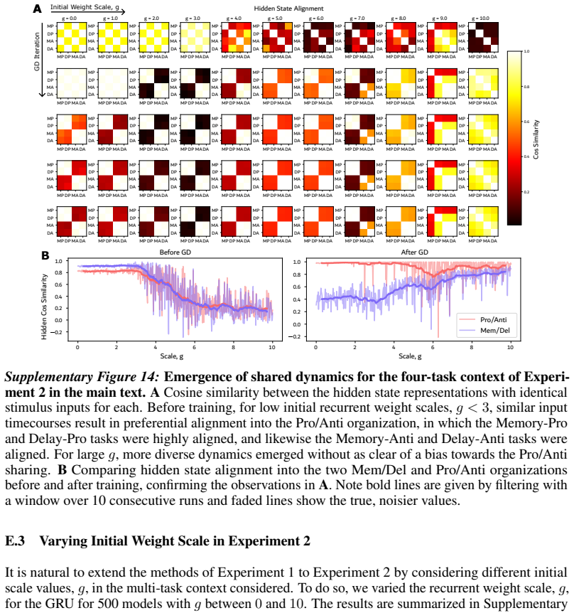
- Sub-task sharing can be predicted early: the off-diagonal blocks $P_i K_{ij} P_j^*$ and the interference matrix $M$ indicate, from the first few iterations, which groups of tasks will end up with aligned activity subspaces, before the alignment is visible in the hidden states themselves.
- The decomposition carries over to any weight-based dynamical model—GRUs, LSTMs, neural ODEs, and biophysical networks such as Hodgkin–Huxley models—so the rank bound on $K$ gives a general formula for when gradient training of a recurrent system will collapse its dynamics.
Reading between the lines
- Editorial inference: the paper's mechanism suggests a design principle the authors only gesture at—architectures that raise the effective rank of $K$ (richer input encoding, higher-dimensional activity, or parameterizations that keep the $J_\theta$ Gram matrices full-rank) should train faster and collapse less; a direct test would compare collapse depth across architectures matched for task but di
- Editorial inference: the block structure of $PKP^*$ could serve as an online diagnostic for continual and transfer learning—computing the interference matrix at each step would reveal which stored tasks are being overwritten before the loss shows it, enabling task-order or reweighting decisions during training.
- Editorial inference: since $K$'s end-of-training rank stabilizes to a similar low value across initializations, the surviving eigenmodes of $K$ may bound the number of distinct attractors or prototypes a trained network can separate, connecting this operator bottleneck to neural collapse in classification networks as a special case.
Editorial analysis
A structured set of objections, weighed in public.
Referee Report
Summary. The paper proposes KPFlow, an operator-theoretic decomposition of the gradient flow that trains recurrent dynamical systems. The central identity, Proposition 1, states that the hidden-state perturbation produced by one gradient step is δz = -[P ◦ K ◦ P*](Err), where K is a parameter-space kernel and P is the linearized flow propagator. The authors apply this decomposition to RNNs and GRUs trained on a memory-pro task, reporting that K has much lower effective rank than P and concluding that this low-rank bottleneck causes dynamic collapse. They also study a four-task multitask setting, using sub-blocks of K and P to define interference matrices that anticipate the alignment of learned representations. The paper includes an implementation package, extensive experiments across initial weight scales and model families (RNNs, GRUs, ReLU RNNs, Hodgkin-Huxley networks), and two theoretical theorems about the rank of K and the structure of P.
Significance. If the central claim holds, KPFlow would provide a useful unifying lens on recurrent-network training, connecting neural tangent kernel ideas with Lyapunov/optimal-control theory and offering practical SVD-based diagnostics for representation collapse. The manuscript has notable strengths: Proposition 1 is an exact, proven gradient-flow identity, not a heuristic fit; the experimental scope is substantial (hundreds of RNN/GRU training runs, multitask sweeps, and several architecture extensions); and the authors provide a PyTorch package with notebooks intended to reproduce the figures. The proposed PP* parameter-free baseline in Appendix B.4 is conceptually valuable even though it is not deployed. However, the paper's headline causal claim—that the low rank of K drives dynamic collapse 'over and above the task'—is not established, because the reported evidence concerns single-step operators rather than cumulative training dynamics and lacks a control experiment. The theoretical results also contain statements that are either unproven or false in the claimed generality. The paper is therefore best viewed as a promising but overclaimed contribution that requires substantial revision.
major comments (4)
- [Section 3.1, Observation 3.1 and Eq. (5)] The conclusion that dynamic collapse is caused by the low rank of K does not follow from the single-step decomposition. At each training step, rank(δz_s) ≤ rank(K_s), but after S steps the hidden state is z_0 + Σ_s δz_s, whose effective dimension is not bounded by the rank of any single K_s; it can grow linearly with S even if every K_s has effective rank about 7. The collapse measured in Figures 2E-G is a property of the final hidden activity, not of a one-step update, so the paper needs an argument or experiment that connects the per-step rank bound to the cumulative state. Furthermore, the low rank of K is partly inherited from the task: for the RNN, K's kernel is the Gram matrix of x(t) and σ(z(t|x)) (Eqs. (9)-(10)), and the memory-pro task uses only two scalar stimuli on a circle. The PP* parameter-free baseline introduced in Appendix B.4 is the natural control, but it is never computed or used. Concretely, the authors should compare hidden-state collapse under PKP* training versus PP* training (or training with K replaced by a high-rank approximation). Without such a control, the claim in the abstract that collapse is a consequence of network structure 'over and above the nature of the underlying task' is not supported.
- [Section 4, Theorem 2 and Appendix D.4] The proof in Appendix D.4 establishes the algebraic factorization P = U V U^{-1} via the semigroup property of the state-transition matrix, but it does not prove the subsequent claim that the full singular values of U are σ_j(t|x) = exp(λ_j(x)t), with λ_j the j-th Lyapunov exponent. For a time-varying or non-normal product of Jacobians, the finite-time singular values of Φ(t,0|x) are not equal to exponentials of the asymptotic Lyapunov exponents; at best one can write σ_j(t) = exp(λ_j^{FT}(t) t) for time-dependent finite-time exponents. If λ_j is intended to be the finite-time exponent, the statement is definitional; if it is intended to be the asymptotic exponent, it is false in general for the RNN/GRU models considered. Since this part of Theorem 2 is used to support the claim that P is high rank and to connect P to Lyapunov theory, it should either be corrected with explicit assumptions (e.g., normal, time-invariant Jacobians) or removed from the theorem statement.
- [Section 4, Theorem 1 and Appendix D.3] Property (3) of Theorem 1 does not follow from the proof and is false in the stated generality. In the notation of Appendix D.3, the kernel of K_j is a(t,x,t0,x0) · D_q f_outer(t|x) D_q f_outer(t0|x0)^T, where a is the Gram kernel of f_inner. The rank of this operator is controlled by the joint variation of D_q f_outer and f_inner, not by the effective dimension of f_inner alone. For example, take f_inner_j to be a constant scalar (effective dimension 1) and D_q f_outer(t|x) to be a time-varying full-rank n×n matrix; then K_j can have rank n, not 1. The proof's statement that the rank is 'bounded above by the effective dimension of f_inner' needs either a strong restriction (such as D_q f_outer being the identity, which covers the RNN and Hodgkin-Huxley examples) or a corrected bound involving both factors. Because Section 4 cites Theorem 1 as the theoretical motivation for the low rank of K, this is a load-bearing issue rather than a cosmetic one.
- [Appendix E.1 and Section 3.1] The experiments train with ADAM, adaptive learning rates, momentum, and gradient clipping, while Proposition 1 is an identity for continuous gradient flow with an infinitesimally small learning rate. Appendix E.1 acknowledges that ADAM's solutions may differ from true gradient flow, but the paper does not verify that the actual finite-step updates along the training trajectory are well approximated by -P K P* Err at each snapshot. The linearization check in Appendix C compares two ways of computing P for small perturbations, which is not the same as validating the composed operator against the real optimizer update. The authors should report, for representative runs, the cosine similarity or relative error between the empirical Δz_s and the operator-predicted δz_s over training. This would directly address whether the K-bottleneck mechanism describes the trajectories that produce Figures 2 and 4.
minor comments (6)
- [Main text after Eq. (7)] The text says 'since K is positive definite (see Theorem 1 below)', but Theorem 1 states that each K_j is positive semi-definite, and K is typically rank-deficient. Please correct this inconsistency.
- [Corollary 1 and Appendix D.2] Corollary 1 is stated for a fixed linear readout Wout, yet the paragraph immediately before says that in this work the output weights are always trained with GD. The proof later notes that training Wout adds a coupled update. Please clarify the status of the corollary and explicitly separate the fixed-readout and trained-readout cases.
- [Figure 3 and throughout] There are several typos: the y-axis in Figure 3 reads '# of Principle Functions' instead of 'Principal Functions'; Appendix B.1 contains 'general detials'; and Section 3.1 says 'drawn as (x, y) coordinates on a a circle' with a doubled article. These should be corrected.
- [Theorem 2 and Appendix B.4] The symbol U is used both for the fundamental operator in Theorem 2 and for the left singular-vector operator in the SVD notation of Appendix B.4. This notation collision is confusing in a paper that relies heavily on SVDs; please disambiguate, for example by calling the fundamental operator Φ or F.
- [Appendix B.1, Eq. (14)] The loss in Eq. (14) is written with an unsquared norm, while the proof of Corollary 1 assumes a squared-error loss. Please make the definition consistent or explain the normalization.
- [Checklist item 8] The checklist states that details of the computer setup are provided in the Appendix, but the appendix text included in this version does not contain such details. Please either add the compute information or revise the checklist answer.
Circularity Check
No significant circularity: the KPFlow decomposition is an exact algebraic identity; the causal interpretation that K drives collapse is an under-supported inference, not a circular reduction.
full rationale
Proposition 1 is derived directly from the adjoint/backpropagation equations in Appendix D.1; the identity δz = −[P K P*](Err) is a consequence of the definitions of P, K, and P*, with no fitted parameter or hidden assumption making the theorem equivalent to its own input. The empirical finding that K has low effective rank is measured independently of the collapse metric, so Observation 3.1 is not a fitted-input-called-prediction case. The paper's 'Consequently' in Observation 3.1 does overreach: a per-step rank bound on δz does not by itself bound the cumulative span of many gradient updates, and the PP* baseline that would isolate K's causal role is defined in Appendix B.4 but not run. That is a causal-inference and completeness gap, not circularity, because the low-rank property of K is not constructed from the collapse outcome. Self-citations (e.g., refs. 4, 5, 17, 24, 34, 36, 54) are used for background, prior empirical context, and implementation techniques; none is the sole load-bearing justification for the central decomposition or for the low-rank observation. Appendix E.1's acknowledgment that ADAM may deviate from true gradient flow is a limitation on external validity, not a circular step. Overall, the derivation chain is self-contained and the paper's main mathematical claims do not reduce to their inputs by definition.
Assumptions & free parameters
assumptions (3)
- domain assumption Discrete GD updates are well approximated by the continuous gradient flow linearized at each step (the operator P).
- domain assumption The model is weight-based, with each weight W_j applied exactly once in a single evaluation of f, enabling the kernel to decompose into a sum of Gram operators.
- standard math Trajectories live in a Hilbert space L^2 over time and trials, and the operators are Hilbert-Schmidt integral operators with well-defined SVDs.
Cite this review
Pith. "Pith review of KPFlow: An Operator Perspective on Dynamic Collapse Under Gradient Descent Training of Recurrent Networks." pith.science (2026). https://pith.science/paper/BDP5V67M
@misc{pith2026250706381,
  author       = {Pith},
  title        = {Pith review of: KPFlow: An Operator Perspective on Dynamic Collapse Under Gradient Descent Training of Recurrent Networks},
  year         = {2026},
  howpublished = {\url{https://pith.science/paper/BDP5V67M}},
  note         = {Machine review of arXiv:2507.06381}
}
read the original abstract
Gradient Descent (GD) and its variants are the primary tool for enabling efficient training of recurrent dynamical systems such as Recurrent Neural Networks (RNNs), Neural ODEs and Gated Recurrent units (GRUs). The dynamics that are formed in these models exhibit features such as neural collapse and emergence of latent representations that may support the remarkable generalization properties of networks. In neuroscience, qualitative features of these representations are used to compare learning in biological and artificial systems. Despite recent progress, there remains a need for theoretical tools to rigorously understand the mechanisms shaping learned representations, especially in finite, non-linear models. Here, we show that the gradient flow, which describes how the model's dynamics evolve over GD, can be decomposed into a product that involves two operators: a Parameter Operator, K, and a Linearized Flow Propagator, P. K mirrors the Neural Tangent Kernel in feed-forward neural networks, while P appears in Lyapunov stability and optimal control theory. We demonstrate two applications of our decomposition. First, we show how their interplay gives rise to low-dimensional latent dynamics under GD, and, specifically, how the collapse is a result of the network structure, over and above the nature of the underlying task. Second, for multi-task training, we show that the operators can be used to measure how objectives relevant to individual sub-tasks align. We experimentally and theoretically validate these findings, providing an efficient Pytorch package, \emph{KPFlow}, implementing robust analysis tools for general recurrent architectures. Taken together, our work moves towards building a next stage of understanding of GD learning in non-linear recurrent models.
Figures


Figures from the paper (4 more)


Reference graph
Works this paper leans on
-
[1]
Chen, Yulia Rubanova, Jesse Bettencourt, and David Duvenaud
Ricky T.Q. Chen, Yulia Rubanova, Jesse Bettencourt, and David Duvenaud. Neural ordinary differential equations. Advances in Neural Information Processing Systems, 31, 2018
work page 2018
-
[2]
Deep learning.Nature, 521(7553):436–444, 2015
Yann LeCun, Yoshua Bengio, and Geoffrey Hinton. Deep learning.Nature, 521(7553):436–444, 2015
2015
-
[3]
Opening the black box: low-dimensional dynamics in high- dimensional recurrent neural networks
David Sussillo and Omri Barak. Opening the black box: low-dimensional dynamics in high- dimensional recurrent neural networks. Neural Computation, 25(3):626–649, 2013
work page 2013
-
[4]
M. Farrell, S. Recanatesi, and E. Shea-Brown. From lazy to rich to exclusive task representations in neural networks and neural codes. Current Opinion in Neurobiology, 83:102780, 2023. Epub 2023 Sep 25
work page 2023
-
[5]
Laura N. Driscoll, Krishna V . Shenoy, and David Sussillo. Flexible multitask computation in recurrent networks utilizes shared dynamical motifs. Nature Neuroscience, 27:1349–1363, 2024
work page 2024
-
[6]
Elia Turner and Omri Barak. The simplicity bias in multi-task rnns: Shared attractors, reuse of dynamics, and geometric representation. In A. Oh, T. Naumann, A. Globerson, K. Saenko, M. Hardt, and S. Levine, editors, Advances in Neural Information Processing Systems , vol- ume 36, pages 25495–25507. Curran Associates, Inc., 2023
work page 2023
-
[7]
The interplay between randomness and structure during learning in rnns
Friedrich Schuessler, Francesca Mastrogiuseppe, Alexis Dubreuil, Srdjan Ostojic, and Omri Barak. The interplay between randomness and structure during learning in rnns. In Advances in Neural Information Processing Systems, volume 33, pages 13352–13362. Curran Associates, Inc., 2020
work page 2020
-
[8]
Pytorch: An imperative style, high-performance deep learning library, 2019
Adam Paszke, Sam Gross, Francisco Massa, Adam Lerer, James Bradbury, Gregory Chanan, Trevor Killeen, Zeming Lin, Natalia Gimelshein, Luca Antiga, Alban Desmaison, Andreas Köpf, Edward Yang, Zach DeVito, Martin Raison, Alykhan Tejani, Sasank Chilamkurthy, Benoit Steiner, Lu Fang, Junjie Bai, and Soumith Chintala. Pytorch: An imperative style, high-performa...
2019
Show all 80 references
-
[9]
Hodgkin and A.F
A.L. Hodgkin and A.F. Huxley. A quantitative description of membrane current and its application to conduction and excitation in nerve. The Journal of physiology, 117(4):449–472, 1952
1952
-
[10]
D. E. Rumelhart, G. E. Hinton, and R. J. Williams. Learning internal representations by error propagation. In Parallel Distributed Processing: Explorations in the Microstructure of Cognition, Volume 1: Foundations, pages 318–362. MIT Press, Cambridge, MA, 1986
1986
-
[11]
Neural machine translation by jointly learning to align and translate, 2016
Dzmitry Bahdanau, Kyunghyun Cho, and Yoshua Bengio. Neural machine translation by jointly learning to align and translate, 2016
2016
-
[12]
van der Schaft
Henk Nijmeijer and Arjan J. van der Schaft. Nonlinear Dynamical Control Systems. Springer, New York, 1990. 10
1990
-
[13]
Neural tangent kernel: Convergence and generalization in neural networks
Arthur Jacot, Franck Gabriel, and Clément Hongler. Neural tangent kernel: Convergence and generalization in neural networks. Advances in Neural Information Processing Systems, 31, 2018
2018
-
[14]
The recurrent neural tangent kernel
Saman Alemohammad, Zhuang Wang, Remi Balestriero, and Richard Baraniuk. The recurrent neural tangent kernel. Advances in Neural Information Processing Systems, 33, 2020
2020
-
[15]
Exploring the impact of activation functions in training neural ODEs
Tianxiang Gao, Siyuan Sun, Hailiang Liu, and Hongyang Gao. Exploring the impact of activation functions in training neural ODEs. In The Thirteenth International Conference on Learning Representations, 2025
2025
-
[16]
Deep residual learning for image recognition, 2015
Kaiming He, Xiangyu Zhang, Shaoqing Ren, and Jian Sun. Deep residual learning for image recognition, 2015
2015
-
[17]
On lyapunov exponents for rnns: Understanding information propagation using dynamical systems tools
Ryan V ogt, Maximilian Puelma Touzel, Eli Shlizerman, and Guillaume Lajoie. On lyapunov exponents for rnns: Understanding information propagation using dynamical systems tools. Frontiers in Applied Mathematics and Statistics, 8, 2022
2022
-
[18]
Haim Sompolinsky, Andrea Crisanti, and Hermann J. Sommers. Chaos in random neural networks. Physical Review Letters, 61(3):259–262, 1988
1988
-
[19]
Kanaka Rajan and L. F. Abbott. Eigenvalue spectra of random matrices for neural networks. Physical Review Letters, 97(18):188104, 2006
2006
-
[20]
David Sussillo and L. F. Abbott. Generating coherent patterns of activity from chaotic neural networks. Neuron, 63(4):544–557, 2009
2009
-
[21]
Zavatone-Veth
Blake Bordelon, Jordan Cotler, Cengiz Pehlevan, and Jacob A. Zavatone-Veth. Dynamically learning to integrate in recurrent neural networks, 2025
2025
-
[22]
Rainer Engelken, Fred Wolf, and L. F. Abbott. Lyapunov spectra of chaotic recurrent neural networks, 2020
2020
-
[23]
Transition to chaos in random neuronal networks
Jonathan Kadmon and Haim Sompolinsky. Transition to chaos in random neuronal networks. Physical Review X, 5(4):041030, 2015
2015
-
[24]
How connectivity structure shapes rich and lazy learning in neural circuits
Yuhan Helena Liu, Aristide Baratin, Jonathan Cornford, Stefan Mihalas, Eric Todd SheaBrown, and Guillaume Lajoie. How connectivity structure shapes rich and lazy learning in neural circuits. In The Twelfth International Conference on Learning Representations, 2024
2024
-
[25]
Organiz- ing recurrent network dynamics by task-computation to enable continual learning
Lea Duncker, Laura Driscoll, Krishna V Shenoy, Maneesh Sahani, and David Sussillo. Organiz- ing recurrent network dynamics by task-computation to enable continual learning. In Advances in Neural Information Processing Systems, volume 33, pages 14387–14397. Curran Associates, I...
2020
-
[26]
Learning representations by back-propagating errors
David E Rumelhart, Geoffrey E Hinton, and Ronald J Williams. Learning representations by back-propagating errors. Nature, 323(6088):533–536, 1986
1986
-
[27]
Kistler, Richard Naud, and Liam Paninski
Wulfram Gerstner, Werner M. Kistler, Richard Naud, and Liam Paninski. Neuronal Dynamics: From Single Neurons to Networks and Models of Cognition. Cambridge University Press, 2014
2014
-
[28]
Mean-field theory of two-layer neural networks: dimension-free bounds and kernel limit
Song Mei, Tomasz Misiakiewicz, and Andrea Montanari. Mean-field theory of two-layer neural networks: dimension-free bounds and kernel limit. Advances in Neural Information Processing Systems, 31, 2018
2018
-
[29]
Context-dependent computation by recurrent dynamics in prefrontal cortex
Valerio Mante, David Sussillo, Krishna V Shenoy, and William T Newsome. Context-dependent computation by recurrent dynamics in prefrontal cortex. Nature, 503(7474):78–84, 2013
2013
-
[30]
Open the black box of recurrent neural network by decoding the internal dynamics
Jiacheng Tang, Hao Yin, and Qi Kang. Open the black box of recurrent neural network by decoding the internal dynamics. In 2022 IEEE International Conference on Networking, Sensing and Control (ICNSC), pages 1–6, 2022
2022
-
[31]
Izhikevich
Eugene M. Izhikevich. Dynamical Systems in Neuroscience: The Geometry of Excitability and Bursting. MIT Press, 2007. 11
2007
-
[32]
Peter Dayan and Laurence F. Abbott. Theoretical Neuroscience: Computational and Mathemat- ical Modeling of Neural Systems. MIT Press, 2001
2001
-
[33]
Exploring flip flop memories and beyond: Training recurrent neural networks with key insights
Carlos Jarne. Exploring flip flop memories and beyond: Training recurrent neural networks with key insights. Frontiers in Systems Neuroscience, 18:1269190, Mar 2024
2024
-
[34]
Gradient-based learning drives robust representations in recurrent neural networks by balancing compression and expansion
Matthew Farrell, Stefano Recanatesi, Timothy Moore, Guillaume Lajoie, and Eric Shea-Brown. Gradient-based learning drives robust representations in recurrent neural networks by balancing compression and expansion. Nature Machine Intelligence, 4(6):564–573, 2022
2022
-
[35]
Vardan Papyan, X. Y . Han, and David L. Donoho. Prevalence of neural collapse during the terminal phase of deep learning training. Proceedings of the National Academy of Sciences, 117(40):24652–24663, 2020
2020
-
[36]
Predictive learning as a network mechanism for extracting low-dimensional latent space representations
Stefano Recanatesi, Matthew Farrell, Guillaume Lajoie, Sophie Deneve, Mattia Rigotti, and Eric Shea-Brown. Predictive learning as a network mechanism for extracting low-dimensional latent space representations. Nature Communications, 12(1):1417, 2021
2021
-
[37]
Pereira, and William Bialek
Naftali Tishby, Fernando C. Pereira, and William Bialek. The information bottleneck method. In Proceedings of the 37th Annual Allerton Conference on Communication, Control, and Computing, pages 368–377, Monticello, IL, USA, 1999
1999
-
[38]
Joglekar, Henry F
Guangyu Robert Yang, Maitham R. Joglekar, Henry F. Song, William T. Newsome, and Xiao- Jing Wang. Task representations in neural networks trained to perform many cognitive tasks. Nature Neuroscience, 22(2):297–306, 2019
2019
-
[39]
Out-of- domain generalization in dynamical systems reconstruction
Niclas Göring, Florian Hess, Manuel Brenner, Zahra Monfared, and Daniel Durstewitz. Out-of- domain generalization in dynamical systems reconstruction. arXiv preprint arXiv:2402.18377, 2024
2024 arXiv
-
[40]
Ergodic theory of differentiable dynamical systems
David Ruelle. Ergodic theory of differentiable dynamical systems. Publications Mathématiques de l’IHÉS, 50:27–58, 1979
1979
-
[41]
Finite-time lyapunov exponents of deep neural networks
L Storm, Hampus Linander, J Bec, Kristian Gustavsson, and Bernhard Mehlig. Finite-time lyapunov exponents of deep neural networks. Physical Review Letters, 132(5):057301, 2024
2024
-
[42]
On the difficulty of learning chaotic dynamics with rnns
Jonas Mikhaeil, Zahra Monfared, and Daniel Durstewitz. On the difficulty of learning chaotic dynamics with rnns. Advances in neural information processing systems , 35:11297–11312, 2022
2022
-
[43]
Y . LeCun. A theoretical framework for back-propagation. In D. Touretzky, G. Hinton, and T. Sejnowski, editors, Neural Information Processing Systems, volume 1, pages 31–39. Morgan Kaufmann Publishers, Inc., San Francisco, CA, 1988
1988
-
[44]
A proposal on machine learning via dynamical systems
Weinan E. A proposal on machine learning via dynamical systems. arXiv preprint arXiv:1711.00579, 2017
2017 arXiv
-
[45]
Maximum principle based algorithms for deep learning
Chen Li, Chun Chen, Chao Tai, and Weinan E. Maximum principle based algorithms for deep learning. arXiv preprint arXiv:1708.01038, 2017
2017 arXiv
-
[46]
Discretize-optimize vs
Derek Onken and Lars Ruthotto. Discretize-optimize vs. optimize-discretize for time-series regression and continuous normalizing flows, 2020
2020
-
[47]
L. S. Pontryagin, V . G. Boltyanskii, R. V . Gamkrelidze, and E. F. Mishchenko.The Mathematical Theory of Optimal Processes. Pergamon Press, 1962. Translated from the Russian original
1962
-
[48]
Golub and Charles F
Gene H. Golub and Charles F. Van Loan. Matrix Computations. Johns Hopkins University Press, 4th edition, 2013
2013
-
[49]
Introductory Functional Analysis with Applications
Erwin Kreyszig. Introductory Functional Analysis with Applications. Wiley, reprint edition, 1989. 12
1989
-
[50]
Oliphant, Matt Haberland, Tyler Reddy, David Cournapeau, Evgeni Burovski, Pearu Peterson, Warren Weckesser, Jonathan Bright, Stéfan J
Pauli Virtanen, Ralf Gommers, Travis E. Oliphant, Matt Haberland, Tyler Reddy, David Cournapeau, Evgeni Burovski, Pearu Peterson, Warren Weckesser, Jonathan Bright, Stéfan J. van der Walt, Matthew Brett, Joshua Wilson, K. Jarrod Millman, Nikolay Mayorov, Andrew R. J. Nelson, E...
2020
-
[51]
JAX: composable transformations of Python+NumPy programs, 2018
James Bradbury, Roy Frostig, Peter Hawkins, Matthew James Johnson, Chris Leary, Dougal Maclaurin, George Necula, Adam Paszke, Jake VanderPlas, Skye Wanderman-Milne, and Qiao Zhang. JAX: composable transformations of Python+NumPy programs, 2018
2018
-
[52]
Paul Frederickson, J. L. Kaplan, E. D. Yorke, and J. A. Yorke. The liapunov dimension of strange attractors. Journal of Differential Equations, 49:185–207, 1983
1983
-
[53]
Pavel Tolmachev and Tatiana A. Engel. Single-unit activations confer inductive biases for emergent circuit solutions to cognitive tasks. bioRxiv, 2024
2024
-
[54]
Evolutionary algorithms as an alternative to backpropagation for supervised training of biophysical neural networks and neural odes
James Hazelden, Yuhan Helena Liu, Eli Shlizerman, and Eric Shea-Brown. Evolutionary algorithms as an alternative to backpropagation for supervised training of biophysical neural networks and neural odes. arXiv preprint arXiv:2311.10869, 2023
2023 arXiv
-
[55]
per-trial trajectories
Emre O. Neftci, Hesham Mostafa, and Friedemann Zenke. Surrogate gradient learning in spiking neural networks, 2019. 13 Appendix to KPFlow Main Text and Appendix Contents 1 Introduction 1 2 Preliminaries 2 2.1 Notation . . . . . . . . . . . . . . . . . . . . . . . . . . . . . ....
2019
-
[56]
Forward propagation, where the state z(t|x) is simulated from time 0 to time tend
-
[57]
Adjoint backpropagation, where an adjoint variable is simulated backwards from time tend to time 0
-
[58]
extrapolating
Gradient backpropagation, where a running gradient is simulated backwards from time tend to time 0 effectively “extrapolating” the adjoint in state space to parameter space sensitivities. Step 1 is as detailed above. Step 2 computes the per-trial adjoint, a(t|d), defined as a(...
-
[59]
direct integral
Running Gradient Supplementary Figure 8: Schematic of the Discretized Adjoint Method for Sequential Models. Step (3) defines a running gradient sensitivity gθ(t|d) in the parameter space, which is typically higher dimensional than the hidden state space. Explicitly, it is give...
-
[60]
The linear approach, using the state-transition matrix definition in Equation 33,
-
[61]
The linear approach relies on the variation of parameters for small inputs q
The direct approach, relying on perturbing the model dynamics and measuring how the hidden state is perturbed. The linear approach relies on the variation of parameters for small inputs q. The linearized form of P produces perturbations δz given changes δf to the tangential dy...
-
[62]
M x t+1 = Jz(t|x) · Qx t ,
-
[63]
View" of Computation Graph Wj Supplementary Figure 9: Visual depiction of computation graph “view
Qx t+1, Rx t+1 =QR(M x t+1), Then, we compute Φ(t, t0|x) = Qx t Rx t Rx t−1 · · ·Rx t0+1Qx t0 for t > t0 and Φ(t, t|x) = Id. Finally, the value of (Pq)(t|x) is given by the state-transition solution Equation 33. This approach is likely more stable since it accounts for very sm...
-
[64]
block arrowhead matrix
From the above, we see that the Jacobian has structure: Dzf = DV fV DmfV DnfV DhfV DV fm Dmfm 0 0 DV fn 0 DV fn 0 DV fh 0 0 DV fh ∈ R4n×4n, (83) where DV fV = diag(gkn4 + gN am3 ⊙ h + gl) + W diag(σ′(V )), (84) DV fk = −diag((α′ k(V ) + β′ k(V )) ⊙ k) (85) Dkfk = −di...
2025
-
[65]
Claims Question: Do the main claims made in the abstract and introduction accurately reflect the paper’s contributions and scope? Answer: [Yes] Justification: Our claims are re-stated in the contributions at the end of the introduction section and outlined in the Experiments a...
-
[66]
Limitations Question: Does the paper discuss the limitations of the work performed by the authors? Answer: [Yes] Justification: Our work’s limitations and future directions are provided in the Discussion section
-
[67]
Theory assumptions and proofs Question: For each theoretical result, does the paper provide the full set of assumptions and a complete (and correct) proof? Answer: [Yes] Justification: Yes, proofs are provided in the Appendix and informal observations are motivated with experi...
-
[68]
Experimental result reproducibility Question: Does the paper fully disclose all the information needed to reproduce the main ex- perimental results of the paper to the extent that it affects the main claims and/or conclusions of the paper (regardless of whether the code and da...
-
[69]
Open access to data and code Question: Does the paper provide open access to the data and code, with sufficient instruc- tions to faithfully reproduce the main experimental results, as described in supplemental material? Answer: [Yes] Justification: Yes, our code is linked in ...
-
[70]
Experimental setting/details Question: Does the paper specify all the training and test details (e.g., data splits, hyper- parameters, how they were chosen, type of optimizer, etc.) necessary to understand the results? Answer: [Yes] Justification: Details are provided in exper...
-
[71]
Experiment statistical significance Question: Does the paper report error bars suitably and correctly defined or other appropriate information about the statistical significance of the experiments? Answer: [Yes] Justification: Error bars are included in plots where relevant an...
-
[72]
Experiments compute resources Question: For each experiment, does the paper provide sufficient information on the com- puter resources (type of compute workers, memory, time of execution) needed to reproduce the experiments? Answer: [Yes] Justification: Details of computer set...
-
[73]
Code of ethics Question: Does the research conducted in the paper conform, in every respect, with the NeurIPS Code of Ethics https://neurips.cc/public/EthicsGuidelines? 33 Answer: [Yes] Justification: The research does conform
-
[74]
Broader impacts Question: Does the paper discuss both potential positive societal impacts and negative societal impacts of the work performed? Answer: [Yes] Justification: Broad discussion of our work to machine learning is provided in the Discussion section
-
[75]
Safeguards Question: Does the paper describe safeguards that have been put in place for responsible release of data or models that have a high risk for misuse (e.g., pretrained language models, image generators, or scraped datasets)? Answer: [NA] Justification: We do not intro...
-
[76]
Licenses for existing assets Question: Are the creators or original owners of assets (e.g., code, data, models), used in the paper, properly credited and are the license and terms of use explicitly mentioned and properly respected? Answer: [Yes] Justification: The paper author...
-
[77]
New assets Question: Are new assets introduced in the paper well documented and is the documentation provided alongside the assets? Answer: [Yes] Justification: The Appendix and main text provide a comprehensive summary of introduced code and methods
-
[78]
Crowdsourcing and research with human subjects Question: For crowdsourcing experiments and research with human subjects, does the paper include the full text of instructions given to participants and screenshots, if applicable, as well as details about compensation (if any)? A...
-
[79]
Institutional review board (IRB) approvals or equivalent for research with human subjects Question: Does the paper describe potential risks incurred by study participants, whether such risks were disclosed to the subjects, and whether Institutional Review Board (IRB) approvals...
-
[80]
Answer: [NA] Justification: LLMs are not a core component of our research and they were not used in generation of the paper
Declaration of LLM usage Question: Does the paper describe the usage of LLMs if it is an important, original, or non-standard component of the core methods in this research? Note that if the LLM is used only for writing, editing, or formatting purposes and does not impact the ...
Reviewed August 6, 2026 · model on record in the stance chip above.
Discussion (0). Continue with ORCID to comment.