REVIEW 5 major objections 5 minor 2 cited by
Time Series Foundation Models for Multivariate Financial Time Series Forecasting
T0 review · 5 major / 5 minor · reviewed 2026-08-06 · deepseek-v4-flash
Pith's one-line read Pretrained time-series foundation models cut financial forecast error by 25–50% on limited data, this study reports.
desk verdict Honest pilot study with a reusable paired pretrained/untrained protocol, but the headline transfer gains are not identified as transfer until the TTM pretraining leakage question is settled. read the letter →
The pith
A machine-rendered reading of the paper's core claim, the machinery that carries it, and where it could break.
The reading
What carries the argument
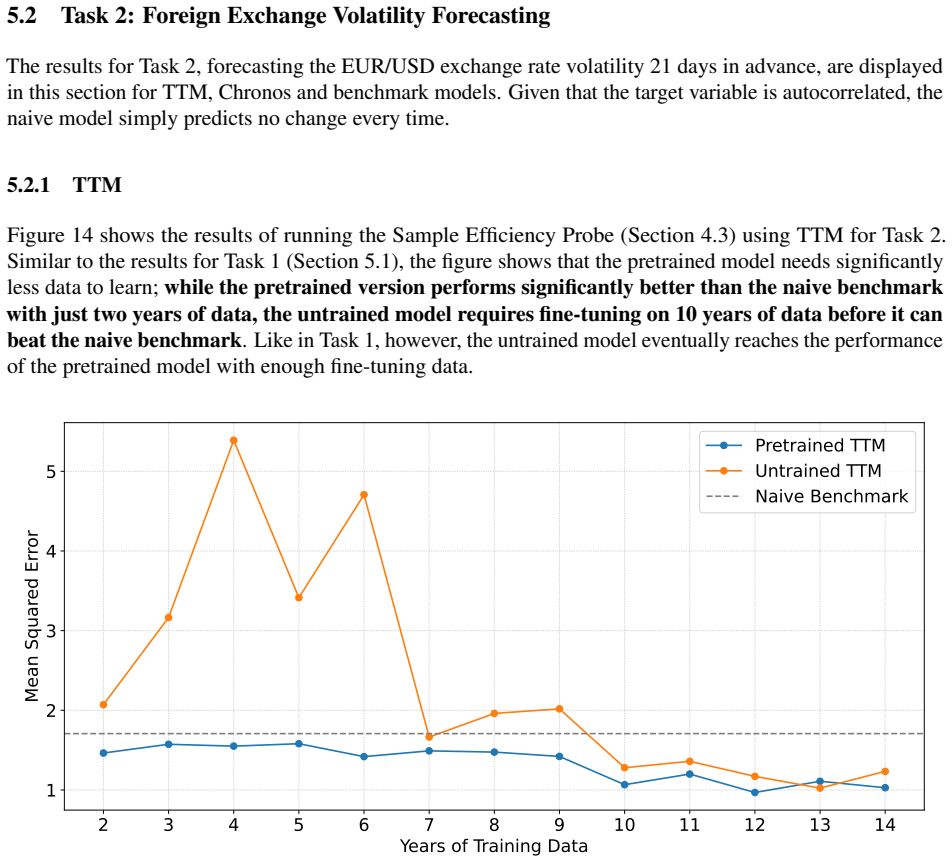
The evaluation rests on two paired experimental protocols. The transfer-gain test compares a pretrained model with a randomly initialised copy of the same architecture in both zero-shot and fine-tuned regimes, measuring relative gains $\Delta_{\mathrm{ZS}}$ and $\Delta_{\mathrm{FT}}$; a positive gain attributes the improvement to pretraining rather than architecture. The sample-efficiency probe trains both variants on incremental amounts of historical data, so the gap between their learning curves quantifies how many years of data pretraining saves. The models themselves are the other load-bearing components: Tiny Time Mixers is a compact MLP-based time-series model pretrained on broad corpora that include Bitcoin data, and Chronos tokenises time series values into quantised bins and trains a language-model-style transformer without financial pretraining data. The paper argues that the contrast between these two models points to pretraining-corpus composition as a key driver of transfer.
What would settle it
Inspect the time stamps of TTM's pretraining datasets, especially the Bitcoin series, against the 2005–2025 evaluation windows; if any pretraining sample falls inside a test window, retrain from scratch on the truncated corpus and check whether the 25–50% gain persists. A second check is to configure TTM with a true 21-day forecast horizon instead of 30, 48, or 96 days and see whether the stated gains still hold.
Extended reading notes
Core claim
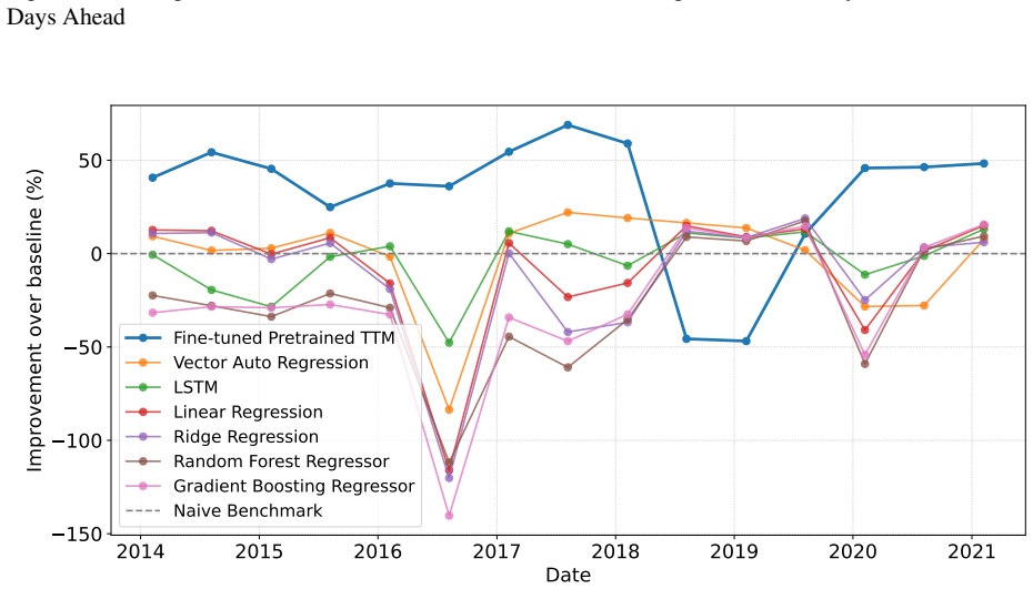
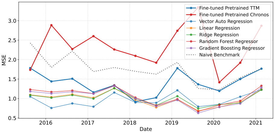
The paper's central claim is that a pretrained TSFM's weights carry reusable temporal structure that transfers to financial forecasting, while an identical architecture trained from scratch must rediscover that structure from limited data. This is established through paired experiments: fine-tuning both a pretrained Tiny Time Mixers model and a randomly initialized copy of the same architecture, then comparing their errors. Across US 10-year Treasury yield changes, EUR/USD realised volatility, and an equity spread between two country indices, the pretrained version achieved 25–50% lower MSE with limited fine-tuning data, 10–30% lower MSE with full data, and consistently needed fewer years of history to reach comparable performance. In the volatility and spread tasks, the pretrained model in zero-shot mode outperformed naive benchmarks, and in the spread task it outperformed all tested benchmark models without any fine-tuning. The paper also finds that traditional specialised models matched or exceeded TTM in two of three tasks, and that Chronos, an LLM-adapted TSFM pretrained without financial data, failed to beat naive baselines in any task.
Load-bearing premise
The clean-transfer conclusion depends on TTM's pretraining corpus not containing data from the same future period as the evaluation windows; if it does, the measured advantage is leakage rather than transfer.
Editorial extensions
If this is right
- If the paper is right, practitioners with fewer than ten years of instrument history should prefer fine-tuning a pretrained TSFM over training an equivalent architecture from scratch.
- Zero-shot TSFM forecasts can beat naive baselines for autocorrelated and mean-reverting financial series, meaning some forecasting value is available before any task-specific training.
- Fine-tuning transfer gains are largest when data are scarce, suggesting the primary practical value of TSFMs lies in data-constrained settings rather than in pushing the accuracy ceiling on long histories.
- Pretraining corpus composition matters: the model pretrained with financial data transferred well, while the model pretrained without financial data did not, supporting a finance-specific pretraining research direction.
- Native time-series architectures may fit financial data better than LLM-adapted designs, although the paper treats this conclusion as tentative because only two models were compared.
Reading between the lines
- If the transfer gains survive leakage checks, the practical consequence is that a general-purpose pretrained model can substitute for years of proprietary financial history, lowering the data barrier for newly listed or illiquid instruments.
- The TTM-versus-Chronos gap suggests that architecture alone is not the explanation; a direct test would be to pretrain the same architecture on corpora that differ only in whether financial series are included.
- The paper's MSE-based evaluation leaves open whether the gains translate into tradeable signals; the appendix backtest on Treasury ETFs points in that direction, but a Sharpe-ratio or directional-accuracy evaluation would settle it.
- A cleaner comparison would align TTM's configured horizons (30, 48, and 96 days) with the stated 21-day task horizons, since a horizon mismatch could distort the measured transfer gains.
Editorial analysis
A structured set of objections, weighed in public.
Referee Report
Summary. The paper evaluates two time-series foundation models, TTM and Chronos-Bolt, on three multivariate financial forecasting tasks: 21-day-ahead US 10-year Treasury yield changes, 21-day-ahead EUR/USD realized volatility, and equity spread forecasts at multiple horizons. The experimental design compares randomly initialized and pretrained versions of the same architecture under both zero-shot and fine-tuned regimes, using paired transfer-gain statistics (Equations 2 and 3) and a sample-efficiency probe that varies the training window length. The central claim is that pretrained TTM fine-tuned on limited financial data achieves 25–50% lower MSE than an identically architected untrained model, requires 3–10 fewer years of data to reach comparable performance, and in some tasks beats naive benchmarks in zero-shot mode. Classical baselines such as VAR, LSTM, ridge regression, and an error-correction model are also compared. The paper concludes that TSFMs are promising for data-constrained financial forecasting but require domain-specific pretraining to be competitive.
Significance. If the headline transfer gains survive a temporally clean evaluation, the paper would make a useful empirical contribution: it defines explicit paired transfer-gain metrics, applies a genuinely interesting pretrained-versus-untrained control for TTM, uses rolling out-of-sample evaluation, and includes a practical backtest in Appendix A.3. The three tasks span different asset classes and statistical properties, and the feature transformations are documented in detail. However, as it stands, the central quantitative claims are not identified as transfer effects because the pretraining corpus may overlap the evaluation period, and the headline numbers rest on single-seed point estimates with no dispersion or significance testing. The horizon configuration also diverges from the stated 21-day task horizon, so the reported MSE values are not measuring exactly what the abstract claims.
major comments (5)
- [2.6.1, Appendix A.1, 6.2] The transfer-gain identification is not established because TTM's pretraining corpus contains financial data whose temporal range is undocumented. Section 2.6.1 and Appendix A.1 list the Bitcoin data set (Zenodo record 5122101) among TTM's pretraining corpora, while the evaluation windows for the sample-efficiency probe and the rolling transfer-gain test run from roughly 2014 through 2024 (Figures 10, 15, and 20). Section 6.2 concedes that 'pretraining from scratch would eliminate potential look-ahead bias from including correlated future data in TTM's financial pretraining dataset.' Since the paper nowhere reports the date range of the Bitcoin record or its relation to the evaluation period, the positive ΔFT and ΔZS values in Tables 10–12 can be produced by temporal leakage rather than by reusable task-agnostic representations. The authors should document non-overlap of the pretraining corpus, use a checkpoint whose pretraining data are verifiably earlier than the evaluation period, or rerun the experiments with a from-scratch pretrained model.
- [4.1.1, Table 8; 1.1; 5] The configured forecast horizons are inconsistent with the stated task horizons, so the reported MSE values are not measuring what the abstract claims. Section 1.1 and Sections 5.1–5.2 describe 21-business-day-ahead forecasts, but Table 8 sets TTM horizons of 30, 48, and 96 for Tasks 1–3; Chronos is run at horizons of 21 and 10 (Table 9). Because MSE is averaged over all forecast steps, the TTM numbers include substantially longer horizons than the naive benchmarks and the Chronos numbers, and the headline 25–50% gains are not directly comparable across models or to the stated 21-day task. This is especially acute in Task 3, where the text reports 5- and 10-day horizons but Table 8 assigns TTM a horizon of 96. The paper should run TTM at the 21-step horizon, report horizon-specific MSE, or provide an explicit argument for why a 30/48/96-step average is equivalent to the stated task.
- [4.1.1, 4.3, Tables 10–12] All results rest on a single fixed seed, and the transfer gains are reported without any measure of dispersion or formal significance test. Section 4.1.1 states that a fixed random seed was used for all TTM experiments, and Tables 10–12 present ΔFT and ΔZS as point estimates. Section 5.4.4 nonetheless describes the gains as 'statistically significant' and 'robust,' but no significance test, confidence interval, or repeated-seed standard error is provided anywhere in the paper. Since the headline claims are quantitative and some of the learning-curve differences in Figures 9, 14, and 19 are modest, the authors should report means and variances over multiple seeds or bootstrap resamples, state the test used, and show error bars in the learning curves.
- [4.3, 5.3.1] The hyperparameter and training-window selection is anchored to a single reference date, and the paper itself documents the resulting overfitting in Task 3. The sample-efficiency probe fixes 22 January 2021 as the reference date and uses it to select the training window k, while Section 4.1.1 says context length, forecast horizon, and epochs were chosen by validation. Section 5.3.1 then notes that performance at that 2021 date shows rough parity between zero-shot and fine-tuned pretrained models and that 'hyperparameter choices and training procedures optimised for January 2021 do not generalise effectively to other time periods.' Because the same k and hyperparameters feed every rolling window in Section 4.4, the rolling transfer gains may partly reflect tuning to a single date. The authors should use a nested or rolling validation protocol, or report sensitivity of the transfer gains to the choice of reference date.
- [5.1.2, 5.2.2, 5.3.2] Chronos is excluded from the transfer-gain analysis after seeing its results, which undercuts the paper's comparison of the two TSFM families. Sections 5.1.2, 5.2.2, and 5.3.2 state that Chronos is excluded from subsequent transfer-gain analyses because it fails to beat the naive benchmark, and the abstract and conclusions nonetheless draw general conclusions about 'TSFMs' and about native time-series architectures versus LLM-adapted approaches from the TTM–Chronos contrast. The authors should report the Chronos ΔFT and ΔZS values even when they are negative, avoid post-hoc exclusion of a model from the primary analysis, or explicitly restrict the conclusions to TTM only.
minor comments (5)
- [5.3.2] The text says 'Figure 16 shows that Chronos fails...' for the Task 3 results, but the Chronos Task 3 results appear in Figure 21; the cross-reference should be corrected.
- [Figures 13, 24, 25] These figures are described as percentage improvement over the naive benchmark but their y-axes are labeled 'MSE'; the axis labels should be changed to 'Improvement over baseline (%).'
- [Figure 10] The y-axis of Figure 10 shows values as low as -400% for 'Improvement over baseline (%)'; the paper should state the exact formula used to compute this quantity and explain how negative values below -100% arise.
- [2.6.1, Table 4] Table 4 and Section 2.6 describe TTM as a multivariate model, but Section 2.6.1 says pretraining is univariate with a channel-independent backbone and that multivariate fine-tuning is optional; the paper should clarify how the multivariate claim applies in zero-shot mode.
- [Throughout] A careful proofread is needed: for example, 'V olatility' appears in several table headers, Section 3.5 contains 'are can also cause jumps,' and Section 2.4.1 begins with an unresolved capital 'An.'
Circularity Check
No significant circularity: the transfer-gain and sample-efficiency results are empirical paired comparisons, not derivations from fitted parameters or load-bearing self-citations.
full rationale
The paper's central claims (25-50% MSE improvements for fine-tuned pretrained TTM over an identically-architected untrained model, 3-10 fewer years of data, and zero-shot wins over naive baselines) are established by direct experiments defined in Sections 2.8.2-2.8.3 and executed in Sections 4.3-4.4. Equations (2) and (3) define transfer gains as relative error differences between two model initialisations on the same data split; they are not identities that make the conclusion true by construction. No parameter is fitted to the evaluation targets and then renamed a prediction; no benchmark result is derived from the claim it is meant to support; and the paper contains no load-bearing self-citation, since the TTM and Chronos references ([63], [64]) are external sources describing the models under test. The acknowledged risk in Section 6.2 that TTM's pretraining corpus includes Bitcoin data (Appendix A.1) and may overlap the 2014-2024 evaluation windows is a temporal-leakage threat to the interpretation of the transfer gains, not a circularity: the pretrained checkpoint is an external artifact, and the paired comparison remains an empirical measurement. If the pretraining data do overlap the evaluation period, the headline numbers would overstate transfer, but that is a validity and correctness concern outside the circularity taxonomy. Horizon mismatches and single-seed runs are similar robustness limitations, not circular reasoning. Accordingly, no circular step can be exhibited with the required quote-and-reduction evidence, and the appropriate score is 0.
Assumptions & free parameters
free parameters (9)
- Transfer-gain decision threshold =
0.1
- Reference date for sample-efficiency probe =
22 January 2021
- TTM forecast horizons =
30 (bond), 48 (FX), 96 (spread)
- TTM context lengths =
90, 512, 512
- TTM epochs =
25 (Task 1), 50 (Task 2), 4 (Task 3)
- Chronos forecast horizons =
21, 21, 10
- Spread normalization window =
42
- VolTransform window =
half-year (approx. 126 business days)
- Naive baseline selection =
zero for changes; previous value for volatility; previous for 5-day spread and zero for 10-day spread
assumptions (6)
- domain assumption The official TTM checkpoint is pretrained on the claimed corpora, including Bitcoin, and is used without modification in zero-shot and fine-tuning.
- domain assumption Temporal causality of the evaluation: the pretraining data do not contain information from the test periods used in this study.
- domain assumption Features aligned at daily frequency from heterogeneous sources (FRED, Yahoo, Macrosynergy, ECB, Investing.com) are correctly merged and stationary after transformations.
- ad hoc to paper MSE averaged over the forecast horizon is the appropriate metric for comparing forecasts at the stated 21-day horizon, even though TTM outputs 30, 48 and 96 steps.
- standard math The ECM-to-AR(1) reduction in Appendix A.4 assumes the short-run adjustment term is zero.
- domain assumption EWA and EWC log prices are cointegrated, so the rolling standardized spread is a valid stationary target.
Cite this review
Pith. "Pith review of Time Series Foundation Models for Multivariate Financial Time Series Forecasting." pith.science (2026). https://pith.science/paper/74Y3IAYN
@misc{pith2026250707296,
  author       = {Pith},
  title        = {Pith review of: Time Series Foundation Models for Multivariate Financial Time Series Forecasting},
  year         = {2026},
  howpublished = {\url{https://pith.science/paper/74Y3IAYN}},
  note         = {Machine review of arXiv:2507.07296}
}
read the original abstract
Financial time series forecasting presents significant challenges due to complex nonlinear relationships, temporal dependencies, variable interdependencies and limited data availability, particularly for tasks involving low-frequency data, newly listed instruments, or emerging market assets. Time Series Foundation Models (TSFMs) offer a promising solution through pretraining on diverse time series corpora followed by task-specific adaptation. This study evaluates two TSFMs (Tiny Time Mixers (TTM) and Chronos) across three financial forecasting tasks: US 10-year Treasury yield changes, EUR/USD volatility, and equity spread prediction. Results demonstrate that TTM exhibits strong transferability. When fine-tuning both the pretrained version of TTM and an untrained model with the same architecture, the pretrained version achieved 25-50% better performance when fine-tuned on limited data and 15-30% improvements even when fine-tuned on lengthier datasets. Notably, TTM's zero-shot performance outperformed naive benchmarks in volatility forecasting and equity spread prediction, with the latter demonstrating that TSFMs can surpass traditional benchmark models without fine-tuning. The pretrained model consistently required 3-10 fewer years of data to achieve comparable performance levels compared to the untrained model, demonstrating significant sample-efficiency gains. However, while TTM outperformed naive baselines, traditional specialised models matched or exceeded its performance in two of three tasks, suggesting TSFMs prioritise breadth over task-specific optimisation. These findings indicate that TSFMs, though still nascent, offer substantial promise for financial forecasting-particularly in noisy, data-constrained tasks-but achieving competitive performance likely requires domain-specific pretraining and architectural refinements tailored to financial time series characteristics.
Figures


Figures from the paper (23 more)






Forward citations
Cited by 2 Pith papers
-
Forecasting Realized Volatility with Time Series Foundation Models: A Comparison with Econometric Benchmarks
Zero-shot time series foundation models largely fail to beat econometric benchmarks for realized volatility forecasting, with only TTM achieving a narrow, calibration-driven edge.
-
Towards Causal Market Simulators
A VAE with a DAG-constrained decoder is proposed to generate counterfactual financial time series; on two synthetic AR(1) models it matches analytical counterfactual probabilities to within 0.03–0.10 L1 error.
Reference graph
Works this paper leans on
-
[1]
R. Adhikari and R. K. Agrawal, “A combination of artificial neural network and random walk models for financial time series forecasting,” Neural Computing and Applications, vol. 24, no. 6, pp. 1441– 1449, 2014, ISSN : 0941-0643. DOI: 10.1007/s00521-013-1386-y
-
[2]
M. Praveen, S. Dekka, D. M. Sai, D. P. Chennamsetty, and D. P. Chinta, “Financial time series forecasting: A comprehensive review of signal processing and optimization-driven intelligent models,” Computational Economics, pp. 1–27, 2025, ISSN : 0927-7099. DOI: 10.1007/s10614-025-108 99-z
-
[3]
Makridakis, “Time series prediction: Forecasting the future and understanding the past andreas s
S. Makridakis, “Time series prediction: Forecasting the future and understanding the past andreas s. weigend and neil a. gershenfeld, eds., 1993, (addison-wesley publishing company, reading, MA, USA), 643 pp., paperback $49.50, ISBN 0-201-62,” International Journal of Forecasting, vol. 10, no. 3, pp. 463–466, 1994, ISSN : 0169-2070. DOI: 10.1016/0169-2070...
-
[4]
Forecasting economic time series using targeted predictors,
J. Bai and S. Ng, “Forecasting economic time series using targeted predictors,” Journal of Economet- rics, vol. 146, no. 2, pp. 304–317, 2008, ISSN : 0304-4076. DOI: 10.1016/j.jeconom.2008.0 8.010
-
[5]
Weather forecasting with ensemble methods,
T. Gneiting and A. E. Raftery, “Weather forecasting with ensemble methods,” Science, vol. 310, no. 5746, pp. 248–249, 2005, ISSN : 0036-8075. DOI: 10.1126/science.1115255
-
[6]
Forecasting energy consumption time series using machine learning techniques based on usage patterns of residential householders,
J.-S. Chou and D. -S. Tran, “Forecasting energy consumption time series using machine learning techniques based on usage patterns of residential householders,” Energy, vol. 165, pp. 709–726, Dec
-
[7]
Forecasting the future: A comprehensive review of time series prediction techniques,
S. Arora Milind Kolambe, “Forecasting the future: A comprehensive review of time series prediction techniques,” Journal of Electrical Systems, vol. 20, no. 2s, pp. 575–586, 2024. DOI: 10.52783/je s.1478
work page doi:10.52783/je 2024
-
[8]
Deep learning-based time series forecasting,
X. Song, L. Deng, H. Wang, Y . Zhang, Y . He, and W. Cao, “Deep learning-based time series forecasting,” Artificial Intelligence Review, vol. 58, no. 1, Nov. 2024, ISSN : 1573-7462. DOI: 10.10 07/s10462-024-10989-8 . [Online]. Available: http://dx.doi.org/10.1007/s104 62-024-10989-8
doi:10.1007/s104 2024
Show all 117 references
-
[9]
Traffic flow prediction with big data: A deep learning approach,
Y . Lv, Y . Duan, W. Kang, Z. Li, and F.-Y . Wang, “Traffic flow prediction with big data: A deep learning approach,” IEEE Transactions on Intelligent Transportation Systems, pp. 1–9, 2014, ISSN : 1558-0016. DOI: 10.1109/tits.2014.2345663. [Online]. Available: http://dx.doi.o ...
2014
-
[10]
A deep learning based stock trading model with 2-d cnn trend detection,
M. U. Gudelek, S. A. Boluk, and A. M. Ozbayoglu, “A deep learning based stock trading model with 2-d cnn trend detection,” in 2017 IEEE Symposium Series on Computational Intelligence (SSCI), IEEE, Nov. 2017, pp. 1–8. DOI: 10.1109/ssci.2017.8285188. [Online]. Available: http://...
2017
-
[11]
Convolutional neural networks for forex time series forecasting,
M. Markova, “Convolutional neural networks for forex time series forecasting,” in EIGHTH IN- TERNATIONAL CONFERENCE NEW TRENDS IN THE APPLICATIONS OF DIFFERENTIAL EQUATIONS IN SCIENCES (NTADES2021), vol. 2459, AIP Publishing, 2022, p. 030 024. DOI: 10 .1063/5.0083533. [Online]...
2022 doi
- [12]
- [13]
- [14]
-
[15]
Learning long-term dependencies with gradient descent is difficult,
Y . Bengio, P. Simard, and P. Frasconi, “Learning long-term dependencies with gradient descent is difficult,” IEEE Transactions on Neural Networks , vol. 5, no. 2, pp. 157–166, 1994. [Online]. Available: https://ieeexplore.ieee.org/document/279181
1994
-
[16]
On the difficulty of training recurrent neural networks,
R. Pascanu, T. Mikolov, and Y . Bengio, “On the difficulty of training recurrent neural networks,” in Proceedings of the 30th International Conference on Machine Learning, 2013, pp. 1310–1318. [Online]. Available: https://proceedings.mlr.press/v28/pascanu13.pdf
2013
-
[17]
Building trend fuzzy granulation-based lstm recurrent neural network for long-term time-series forecasting,
Y . Tang, F. Yu, W. Pedrycz, X. Yang, J. Wang, and S. Liu, “Building trend fuzzy granulation-based lstm recurrent neural network for long-term time-series forecasting,”IEEE Transactions on Fuzzy Systems, vol. 30, no. 6, pp. 1599–1613, Jun. 2022, ISSN : 1941-0034. DOI: 10.1109/...
2022
-
[18]
Assessment of deep recurrent neural network-based strategies for short-term building energy predictions,
C. Fan, J. Wang, W. Gang, and S. Li, “Assessment of deep recurrent neural network-based strategies for short-term building energy predictions,” Applied Energy, vol. 236, pp. 700–710, Feb. 2019, ISSN : 0306-2619. DOI: 10.1016/j.apenergy.2018.12.004 . [Online]. Available: http:/...
2019 doi
- [19]
- [20]
- [21]
- [22]
-
[23]
Adversarial sparse transformer for time series forecasting,
S. Wu, X. Xiao, Q. Ding, P. Zhao, Y . Wei, and J. Huang, “Adversarial sparse transformer for time series forecasting,” inAdvances in Neural Information Processing Systems, H. Larochelle, M. Ranzato, R. Hadsell, M. Balcan, and H. Lin, Eds., vol. 33, Curran Associates, Inc., 202...
2020
-
[24]
Anomaly transformer: Time series anomaly detection with association discrepancy,
J. Xu, H. Wu, J. Wang, and M. Long, “Anomaly transformer: Time series anomaly detection with association discrepancy,” inProceedings of the International Conference on Learning Representations (ICLR), 2022. [Online]. Available: https://openreview.net/forum?id=LzQQ89U1qm_
2022
- [25]
- [26]
-
[27]
A systematic review for transformer-based long-term series forecasting,
L. Su, X. Zuo, R. Li, X. Wang, H. Zhao, and B. Huang, “A systematic review for transformer-based long-term series forecasting,” Artificial Intelligence Review, vol. 58, no. 3, Jan. 2025, ISSN : 1573-
2025
- [28]
-
[29]
J. Ye, W. Zhang, K. Yi,et al., A survey of time series foundation models: Generalizing time series representation with large language model, 2024. DOI: 10.48550/arxiv.2405.02358. eprint: 2405.02358
2024 doi
-
[30]
Does the performance of banking sector promote economic growth? a time series analysis,
K. Reddy, S. Mubeen, K. H. H. Raju, J. V ., and M. B. S., “Does the performance of banking sector promote economic growth? a time series analysis,” International Journal of Professional Business Review, vol. 8, no. 6, e02128, Jun. 2023, ISSN : 2525-3654. DOI: 10.26668/business...
2023 doi
- [31]
-
[32]
Baltruˇsaitis, C
T. Baltruˇsaitis, C. Ahuja, and L.-P. Morency, Multimodal machine learning: A survey and taxonomy,
-
[33]
Deep unsupervised domain adaptation with time series sensor data: A survey,
Y . Shi, X. Ying, and J. Yang, “Deep unsupervised domain adaptation with time series sensor data: A survey,”Sensors, vol. 22, no. 15, p. 5507, Jul. 2022,ISSN : 1424-8220. DOI: 10.3390/s22155507. [Online]. Available: http://dx.doi.org/10.3390/s22155507
2022 doi
-
[34]
Language models are unsuper- vised multitask learners,
A. Radford, J. Wu, R. Child, D. Luan, D. Amodei, and I. Sutskever, “Language models are unsuper- vised multitask learners,” OpenAI, 2019. [Online]. Available: https://cdn.openai.com/bet ter-language-models/language_models_are_unsupervised_multitask_lea rners.pdf
2019
- [35]
-
[36]
E. J. Hu, Y . Shen, P. Wallis,et al., Lora: Low-rank adaptation of large language models, arXiv preprint arXiv:2106.09685, 2021. [Online]. Available: https://arxiv.org/pdf/2106.09685
2021 arXiv
- [37]
- [38]
-
[39]
Large language models for financial aid in financial time-series forecasting,
M. K. Islam, A. Karmacharya, T. Sue, and J. Fox, “Large language models for financial aid in financial time-series forecasting,” in 2024 IEEE International Conference on Big Data (BigData), IEEE, Dec. 2024, pp. 4892–4895. DOI: 10.1109/bigdata62323.2024.10824953. [Online]. Avai...
2024
-
[40]
A decoder-only foundation model for time-series forecasting,
A. Das, W. Kong, R. Sen, and Y . Zhou, “A decoder-only foundation model for time-series forecasting,” arXiv preprint arXiv:2310.10688, 2024. [Online]. Available: https://arxiv.org/abs/2310 .10688
2024 arXiv
- [41]
- [42]
-
[43]
Anomaly detection for vietnamese financial market,
Q. T. Huynh, T. H. Nguyen, D. T. Vu, and M. M. Ngo, “Anomaly detection for vietnamese financial market,” in 2024 18th International Conference on Advanced Computing and Analytics (ACOMPA), IEEE, Nov. 2024, pp. 58–62. DOI: 10.1109/acompa64883.2024.00016. [Online]. Available: ht...
2024
-
[44]
Q. Wen, L. Sun, F. Yang,et al., Time series data augmentation for deep learning: A survey, arXiv preprint arXiv:2002.12478, 2020. [Online]. Available: https://arxiv.org/pdf/2002.124 78
2002 arXiv
-
[45]
Predicting extreme financial risks on imbalanced dataset: A combined kernel fcm and kernel smote based svm classifier,
X. Huang, C.-Z. Zhang, and J. Yuan, “Predicting extreme financial risks on imbalanced dataset: A combined kernel fcm and kernel smote based svm classifier,” Computational Economics, vol. 56, pp. 187–216, 2020. DOI: 10.1007/s10614-020-09975-3 . [Online]. Available: https://l in...
2020 doi
-
[46]
Learning with imbalanced data in smart manufacturing: A comparative study,
Y . Fathy, M. Jaber, and A. Brintrup, “Learning with imbalanced data in smart manufacturing: A comparative study,” IEEE Access, vol. 9, pp. 2734–2757, 2021. [Online]. Available: https://iee explore.ieee.org/document/9309288
2021
-
[47]
A deep learning based expert framework for portfolio prediction and forecasting,
F. Jeribi, R. J. Martin, R. Mittal, et al., “A deep learning based expert framework for portfolio prediction and forecasting,” IEEE Access, vol. 12, pp. 103 810–103 829, 2024. DOI: 10 . 1109 /ACCESS.2024.3434528. [Online]. Available: https://ieeexplore.ieee.org/docu ment/10613392
2024
-
[48]
Transfer learning for class imbalance problems with inadequate data,
S. Al-Stouhi and C. K. Reddy, “Transfer learning for class imbalance problems with inadequate data,” Knowledge and Information Systems, vol. 48, no. 1, pp. 201–228, 2016. DOI: 10.1007/s10115- 015-0870-3 . [Online]. Available: https://link.springer.com/article/10.1007 /s10115-0...
2016 doi
-
[49]
A survey on transfer learning,
S. J. Pan and Q. Yang, “A survey on transfer learning,” IEEE Transactions on Knowledge and Data Engineering, vol. 22, no. 10, pp. 1345–1359, 2010. DOI: 10.1109/TKDE.2009.191. [Online]. Available: https://ieeexplore.ieee.org/document/5288526
2010
-
[50]
A brief review of domain adaptation,
A. Farahani, S. V oghoei, K. Rasheed, and H. R. Arabnia, “A brief review of domain adaptation,” in Advances in Data Science and Information Engineering, ser. Transactions on Computational Science and Computational Intelligence, 2021. DOI: 10.1007/978-3-030-71704-9_65 . [Online...
2021 doi
-
[51]
A novel deep transfer learning framework with adversarial domain adaptation: Application to financial time-series forecasting,
D. Zhang, R. Lin, T. Wei, L. Ling, and J. Huang, “A novel deep transfer learning framework with adversarial domain adaptation: Application to financial time-series forecasting,” Neural Computing and Applications, vol. 35, pp. 24 037–24 054, 2023.DOI: 10.1007/s00521-023-09047-1
2023 doi
- [52]
- [53]
-
[54]
Long short-term memory,
S. Hochreiter and J. Schmidhuber, “Long short-term memory,” Neural Computation, vol. 9, no. 8, pp. 1735–1780, Nov. 1997, ISSN : 1530-888X. DOI: 10.1162/neco.1997.9.8.1735. [Online]. Available: http://dx.doi.org/10.1162/neco.1997.9.8.1735
1997 doi
- [55]
-
[56]
Deep learning for time series classification: A review,
H. Ismail Fawaz, G. Forestier, J. Weber, L. Idoumghar, and P.-A. Muller, “Deep learning for time series classification: A review,” Data Mining and Knowledge Discovery, vol. 33, no. 4, pp. 917–963, Mar. 2019, ISSN : 1573-756X. DOI: 10.1007/s10618- 019- 00619- 1 . [Online]. Avai...
2019 doi
-
[57]
Temporal fusion transformers for interpretable multi- horizon time series forecasting,
B. Lim, S. ¨O. Arık, N. Loeff, and T. Pfister, “Temporal fusion transformers for interpretable multi- horizon time series forecasting,” International Journal of Forecasting, vol. 37, no. 4, pp. 1748– 1764, Oct. 2021, ISSN : 0169-2070. DOI: 10.1016/j.ijforecast.2021.03.012. [On...
2021 doi
- [58]
- [59]
- [60]
- [61]
- [62]
-
[63]
Tiny time mixers (TTMs): Fast pre-trained models for enhanced zero/few-shot forecasting of multivariate time series,
V . Ekambaram, A. Jati, P. Dayama,et al., “Tiny time mixers (TTMs): Fast pre-trained models for enhanced zero/few-shot forecasting of multivariate time series,” arXiv, 2024. DOI: 10.48550/arx iv.2401.03955. eprint: 2401.03955
- [64]
-
[65]
Moment: A family of open time-series foundation models,
M. Goswami, K. Szafer, A. Choudhry, Y . Cai, S. Li, and A. Dubrawski, “Moment: A family of open time-series foundation models,” in International Conference on Machine Learning, 2024
2024
-
[66]
A. W. Services, Chronos-t5-small, hugging face model card, https://huggingface.co/ama zon/chronos-t5-small, Accessed: 2025-05-15, 2024
2025
- [67]
- [68]
- [69]
-
[70]
Adik, PEFT (Parameter-Efficient Fine-Tuning), https://medium.com/@kanikaadik07 /peft-parameter-efficient-fine-tuning-55e32c60c799 , Accessed: 2025-04-12, 2023
K. Adik, PEFT (Parameter-Efficient Fine-Tuning), https://medium.com/@kanikaadik07 /peft-parameter-efficient-fine-tuning-55e32c60c799 , Accessed: 2025-04-12, 2023
2025
- [71]
-
[72]
E. B. Zaken, S. Ravfogel, and Y . Goldberg,Bitfit: Simple parameter-efficient fine-tuning for transformer- based masked language-models, 2021. DOI: 10.48550/ARXIV.2106.10199. [Online]. Avail- able: https://arxiv.org/abs/2106.10199
2021 doi
- [73]
- [74]
-
[75]
C. Li, H. Farkhoor, R. Liu, and J. Yosinski,Measuring the intrinsic dimension of objective landscapes,
- [76]
- [77]
- [78]
- [79]
- [80]
- [81]
-
[82]
X. Liu, Y . Zheng, Z. Du,et al., Gpt understands, too, 2021. DOI: 10.48550/ARXIV.2103.103
2021 doi
-
[83]
A review on transferability estimation in deep transfer learning,
Y . Xue, R. Yang, X. Chen, W. Liu, Z. Wang, and X. Liu, “A review on transferability estimation in deep transfer learning,” IEEE Transactions on Artificial Intelligence, vol. 5, no. 12, pp. 5894– 5914, Dec. 2024, ISSN : 2691-4581. DOI: 10.1109/tai.2024.3445892. [Online]. Avail...
2024
-
[84]
A cointegration analysis of treasury bill yields,
A. D. Hall, H. M. Anderson, and C. W. J. Granger, “A cointegration analysis of treasury bill yields,” The Review of Economics and Statistics, vol. 74, no. 1, p. 116, Feb. 1992, ISSN : 0034-6535. DOI: 10.2307/2109549. [Online]. Available: http://dx.doi.org/10.2307/2109549
1992 doi
- [85]
-
[86]
A no-arbitrage vector autoregression of term structure dynamics with macroeconomic and latent variables,
A. Ang and M. Piazzesi, “A no-arbitrage vector autoregression of term structure dynamics with macroeconomic and latent variables,” Journal of Monetary Economics, vol. 50, no. 4, pp. 745–787, May 2003, ISSN : 0304-3932. DOI: 10.1016/s0304-3932(03)00032-1. [Online]. Available: h...
2003 doi
-
[87]
Price forecast of treasury bond market yield: Optimize method based on deep learning model,
W. Ping, Y . Hu, and L. Luo, “Price forecast of treasury bond market yield: Optimize method based on deep learning model,” IEEE Access, vol. 12, pp. 194 521–194 539, 2024,ISSN : 2169-3536. DOI: 10.1109/access.2024.3519438. [Online]. Available: http://dx.doi.org/10.1109 /ACCESS...
2024
-
[88]
Available: https://arxiv.org/abs/2103.10385
[Online]. Available: https://arxiv.org/abs/2103.10385. 59
-
[89]
Department of the Treasury, Daily treasury par yield curve rates, 2025
U.S. Department of the Treasury, Daily treasury par yield curve rates, 2025. [Online]. Available: https://home.treasury.gov/resource-center/data-chart-center/inter est-rates/TextView?type=daily_treasury_yield_curve
2025
-
[90]
Louis, Federal reserve economic data (fred), Accessed: 2025-05-22,
Federal Reserve Bank of St. Louis, Federal reserve economic data (fred), Accessed: 2025-05-22,
2025
-
[91]
Forecasting interest rates,
G. Duffee, “Forecasting interest rates,” in Handbook of Economic Forecasting . Elsevier, 2013, pp. 385–426. DOI: 10 . 1016 / b978 - 0 - 444 - 53683 - 9 . 00007 - 4. [Online]. Available: http://dx.doi.org/10.1016/B978-0-444-53683-9.00007-4
2013 doi
-
[92]
Forecasting volatility in financial markets: A review,
S.-H. Poon and C. W. J. Granger, “Forecasting volatility in financial markets: A review,”Journal of Economic Literature, vol. 41, no. 2, pp. 478–539, Jun. 2003, ISSN : 0022-0515. DOI: 10.1257/jel .41.2.478. [Online]. Available: http://dx.doi.org/10.1257/jel.41.2.478
2003 doi
-
[93]
Chapter 49 arch models,
T. Bollerslev, R. F. Engle, and D. B. Nelson, “Chapter 49 arch models,” inHandbook of Econometrics. Elsevier, 1994, pp. 2959–3038, ISBN : 9780444887665. DOI: 10.1016/s1573-4412(05)8001 8-2. [Online]. Available: http://dx.doi.org/10.1016/S1573-4412(05)80018-2
1994 doi
- [94]
-
[95]
The volatility of realized volatility,
F. Corsi, S. Mittnik, C. Pigorsch, and U. Pigorsch, “The volatility of realized volatility,”Econometric Reviews, vol. 27, no. 1–3, pp. 46–78, Feb. 2008, ISSN : 1532-4168. DOI: 10.1080/07474930701 853616. [Online]. Available: http://dx.doi.org/10.1080/07474930701853616
2008 doi
-
[96]
Realized volatility forecasting with neural networks,
A. Bucci, “Realized volatility forecasting with neural networks,” Journal of Financial Econometrics, vol. 18, no. 3, pp. 502–531, 2020, ISSN : 1479-8417. DOI: 10 . 1093 / jjfinec / nbaa008. [Online]. Available: http://dx.doi.org/10.1093/jjfinec/nbaa008. 60
2020 doi
-
[97]
A forecast comparison of volatility models: Does anything beat a garch(1, 1)?
P. R. Hansen and A. Lunde, “A forecast comparison of volatility models: Does anything beat a garch(1, 1)?” SSRN Electronic Journal, 2001, ISSN : 1556-5068. DOI: 10.2139/ssrn.264571. [Online]. Available: http://dx.doi.org/10.2139/ssrn.264571
2001 doi
-
[98]
Ltd., Quantamental indicators on jpmaqs, Accessed: 2025-05-22, 2025
M. Ltd., Quantamental indicators on jpmaqs, Accessed: 2025-05-22, 2025. [Online]. Available: htt ps://macrosynergy.com/academy/quantamental-indicators-on-jpmaqs/
2025
-
[99]
[Online]
European Central Bank, Ecb data portal, 2025. [Online]. Available: https://data.ecb.euro pa.eu/data/datasets
2025
-
[100]
[Online]
Investing.com, Investing.com – financial markets worldwide, 2025. [Online]. Available: https: //www.investing.com
2025
-
[101]
Modeling and forecasting realized volatility,
T. G. Andersen, T. Bollerslev, F. X. Diebold, and P. Labys, “Modeling and forecasting realized volatility,” Econometrica, vol. 71, no. 2, pp. 579–625, Mar. 2003, ISSN : 1468-0262. DOI: 10.1111 /1468-0262.00418. [Online]. Available: http://dx.doi.org/10.1111/1468-0262 .00418
2003
-
[102]
Pairs trading on international etfs,
P. Schizas, D. D. Thomakos, and T. Wang, “Pairs trading on international etfs,” SSRN Electronic Journal, 2011, ISSN : 1556-5068. DOI: 10.2139/ssrn.1958546 . [Online]. Available: http: //dx.doi.org/10.2139/ssrn.1958546
2011 doi
-
[103]
Pairs trading: Performance of a relative value arbitrage rule,
E. G. Gatev, W. N. Goetzmann, and K. G. Rouwenhorst, “Pairs trading: Performance of a relative value arbitrage rule,” SSRN Electronic Journal, 2006, ISSN : 1556-5068. DOI: 10.2139/ssrn.141615. [Online]. Available: http://dx.doi.org/10.2139/ssrn.141615
2006 doi
-
[104]
Zhu, Examining pairs trading profitability, Senior essay submitted to the Department of Economics, Yale University., 2024
X. Zhu, Examining pairs trading profitability, Senior essay submitted to the Department of Economics, Yale University., 2024. [Online]. Available:https://economics.yale.edu/sites/defa ult/files/2024-05/Zhu_Pairs_Trading.pdf
2024
-
[105]
Answering the skeptics: Yes, standard volatility models do provide accurate forecasts,
T. G. Andersen and T. Bollerslev, “Answering the skeptics: Yes, standard volatility models do provide accurate forecasts,” International Economic Review, vol. 39, no. 4, p. 885, Nov. 1998, ISSN : 0020-
1998
-
[106]
Costa and R
M. Costa and R. Sueppel,Cross-country equity risk allocation with statistical learning, 2025. [Online]. Available: https://macrosynergy.com/research/cross-country-equity-risk -allocation-with-statistical-learning/
2025
-
[107]
Smith, Cointegrated etf pairs part ii, 2017
C. Smith, Cointegrated etf pairs part ii, 2017. [Online]. Available: https://quantoisseur.c om/2017/01/20/cointegrated-etf-pairs-part-ii/
2017
- [108]
-
[109]
On the estimation of security price volatilities from historical data,
M. B. Garman and M. J. Klass, “On the estimation of security price volatilities from historical data,” The Journal of Business, vol. 53, no. 1, p. 67, Jan. 1980, ISSN : 1537-5374. DOI: 10.1086/296072. [Online]. Available: http://dx.doi.org/10.1086/296072
1980 doi
-
[113]
Mitchell, How to use a pairs trading strategy with etfs, 2015
C. Mitchell, How to use a pairs trading strategy with etfs, 2015. [Online]. Available: https://et fdb.com/etf-trading-strategies/how-to-use-a-pairs-trading-strateg y-with-etfs/
2015
- [117]
-
[723]
Available: http://dx.doi.org/10.1109/TFUZZ.2021.3062723
[Online]. Available: http://dx.doi.org/10.1109/TFUZZ.2021.3062723
2021
- [2017]
-
[2018]
DOI: 10.1016/j.energy.2018.09.144
2018 doi
-
[2025]
Available: https://fred.stlouisfed.org
[Online]. Available: https://fred.stlouisfed.org
- [6598]
-
[7462]
[Online]
DOI: 10.1007/s10462-024-11044-2 . [Online]. Available: http://dx.doi.org /10.1007/s10462-024-11044-2
Reviewed August 6, 2026 · model on record in the stance chip above.
Discussion (0). Sign in to comment.