REVIEW 4 major objections 7 minor 18 references
Modernizing CNN-based Weather Forecast Model towards Higher Computational Efficiency
T0 review · 4 major / 7 minor · reviewed 2026-08-06 · deepseek-v4-flash
Pith's one-line read KAI-α, a 7-million-parameter CNN trained in 12 hours on one GPU, reports lower medium-range forecast RMSE than Pangu-Weather, GraphCast, and IFS HRES.
desk verdict An efficient and plausible CNN forecast model, but the headline accuracy comparison is undermined by an uncontrolled resolution mismatch and inconsistent reported numbers. read the letter →
The pith
A machine-rendered reading of the paper's core claim, the machinery that carries it, and where it could break.
The reading
What carries the argument
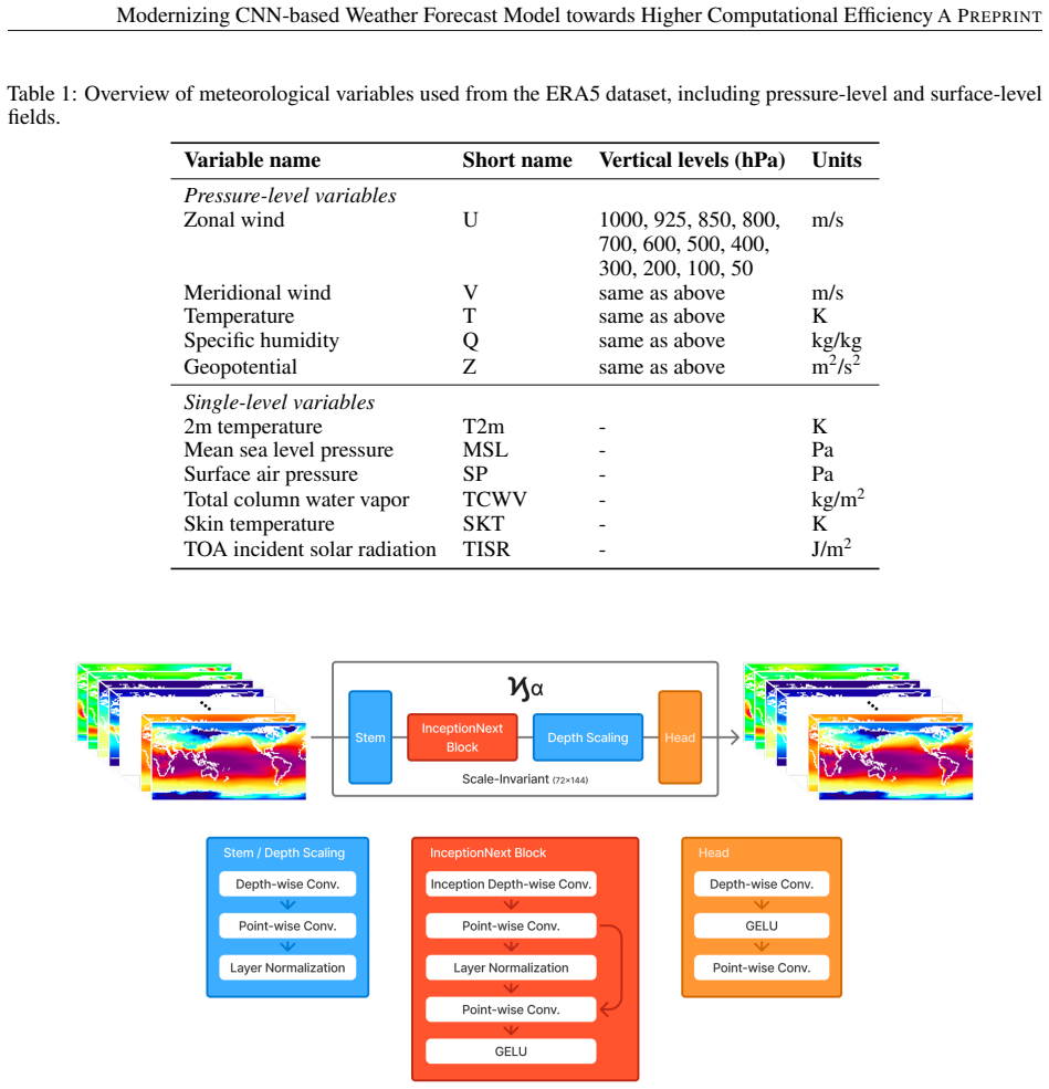
The load-bearing mechanism is a scale-invariant, InceptionNeXt-style convolutional block adapted to spherical grid data. InceptionNeXt is a convolutional token mixer that splits channels into four parallel branches: a small $3\times3$ convolution, two orthogonal band convolutions ($1\times11$ and $11\times1$), and an identity branch; the branches are concatenated and combined in a residual framework, giving a wide receptive field at low FLOPs. The model wraps this block in geocyclic padding, which circularly pads the longitude axis and reorders pole rows so that convolution does not break spherical continuity, and in a scale-invariant structure that holds the 72×144 resolution through all stages instead of downsampling and upsampling. Together these choices let a 7-million-parameter network approximate long-range teleconnections, which the paper describes as pseudo-global attention. The rest of the machinery is deliberately light: depthwise separable stem and head, pointwise convolution for channel mixing, GELU activation, and a latitude-weighted RMSE loss that gives each latitude band its proper area weight.
What would settle it
Recompute RMSE and ACC for all four models on KAI-α's native 2.5° grid, or decompose forecast error by spherical-harmonic wavenumber; if KAI-α's advantage shrinks or reverses once short-wavelength features are scored, the bilinear interpolation step is responsible for the headline skill gap.
Extended reading notes
Core claim
On the paper's own terms, the central discovery is that a careful re-engineering of a CNN baseline yields state-of-the-art forecast skill at a tiny computational budget. KAI-α ingests 67 daily ERA5 variables on a 72×144 (2.5°) grid, passes them through four InceptionNeXt-based stages that keep the full resolution throughout, and is trained for 150 epochs in about 12 hours on one NVIDIA L40s GPU, reaching roughly 7 million parameters. In the 2018 test period the paper reports lower RMSE than Pangu-Weather, GraphCast, and IFS HRES for almost all variables and lead times, with the largest gap at days 7–10, and ACC above the 0.5 skill threshold through days 7–9. The ablation study credits the gains to macro structure, GELU, geocyclic padding, and the scale-invariant scheme in that order. The paper therefore claims that efficient convolutional architectures are a practical alternative to attention-heavy weather models, not merely a lightweight compromise.
Load-bearing premise
The load-bearing premise is that KAI-α's 2.5-degree forecasts, bilinearly interpolated up to the 1.5-degree evaluation grid, can be fairly compared with Pangu-Weather, GraphCast, and IFS HRES outputs at their native higher resolution; if that smoothing hides small-scale errors the other models are penalized for, the reported accuracy advantage is an artifact of the comparison.
Editorial extensions
If this is right
- A roughly 7-million-parameter model can be trained in hours on one GPU, which makes retraining or fine-tuning on new reanalysis data a routine experiment rather than a supercomputer-scale project.
- The ablation results imply that the headline skill comes from the combination of wide receptive fields, spherical padding, and keeping full spatial resolution, so each design choice is reusable and testable independently on other gridded Earth-system tasks.
- If the RMSE comparison is accurate, the main AI forecast baselines can be beaten with far smaller models, changing the cost equation for operational deployment in lower-resource settings.
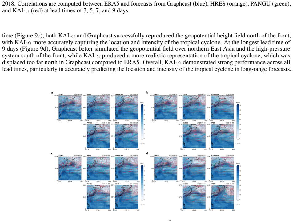
- The two case studies suggest the model captures the large-scale dynamical drivers of the 2018 European heatwave and East Asian monsoon precipitable water and tropical cyclone evolution, not only climatological mean accuracy.
Reading between the lines
- An external check on the central claim would be a fair-grid comparison: evaluating all models at KAI-α's native 2.5° resolution, or decomposing error by wavelength, to see whether the reported advantage survives without the bilinear smoothing step.
- The architecture suggests a transferable template: lightweight CNNs with wide band convolutions and spherical padding may serve as strong, cheap baselines for other gridded geophysical forecasting problems such as ocean, sea-ice, or coupled climate emulation.
- A natural next test is whether the same design retains its efficiency-accuracy balance at higher spatial resolution or on hourly data, where the scale-invariant no-downsampling choice becomes more expensive.
- The extreme-event results are single-event narratives; a multi-case climatological evaluation of heatwaves and tropical cyclones would show whether the 2018 cases are representative.
Editorial analysis
A structured set of objections, weighed in public.
Referee Report
Summary. The paper introduces KAI-α, a lightweight CNN-based global weather forecasting model. It is trained on daily 2.5° ERA5 data with 67 variables, uses about 7 million parameters, and is claimed to train in 12 hours on a single NVIDIA L40s GPU. The authors propose a 'modernization roadmap' from the Weyn et al. (2020) CNN baseline, with macro, micro, and meta design components: a scale-invariant architecture, InceptionNeXt blocks, geocyclic padding, GELU activations, and pointwise channel mixing. The central accuracy claim is that KAI-α matches or exceeds Pangu-Weather, GraphCast, and IFS HRES in RMSE over 10 forecast days (Section 3.2, Figure 4), with additional ACC skill curves and two case studies (European heatwave and East Asian monsoon). The paper emphasizes the practical value of a low-cost, CNN-based alternative to large transformer models.
Significance. If the headline accuracy claim were established, this would be a valuable contribution: a ~7M-parameter weather model trainable on a single GPU that is competitive with 36M–256M parameter transformer-based systems would be a meaningful step toward accessible, efficient AI weather forecasting. The paper's positive features include a systematic ablation of design choices, comparisons against external WeatherBench2 baselines, and concrete case studies. However, the significance is currently limited by the evaluation protocol. The RMSE comparison in Section 3.2 is not controlled for native resolution or temporal aggregation, and the GFLOPs/ACC numbers in Section 3.1 are internally inconsistent. Because these issues bear directly on the paper's central claims of 'competitive accuracy' and 'computational efficiency,' the result cannot yet be taken at face value. The paper also does not release code or trained checkpoints, which would be important for reproducibility and for verifying the WeatherBench2 comparison protocol.
major comments (4)
- [§3.2, Figure 4] The comparison with Pangu-Weather, GraphCast, and HRES is confounded by differences in native resolution and interpolation. The text states that KAI-α's 2.5° outputs are bilinearly interpolated to the 1.5° target grid, while the baselines have higher native resolutions before regridding. Bilinear upsampling acts as a low-pass filter that suppresses small-scale forecast errors, especially the 'double penalty' from slightly mislocated features, and can therefore reduce RMSE even when the underlying large-scale skill is not superior. To establish the claim that KAI-α 'exhibits lower RMSE than the other models,' the authors must control the effective resolution of all models, for example by coarsening every forecast to 2.5° before interpolating to the common grid, or by reporting spectral skill scores.
- [§3.2] The temporal sampling of the comparison is not specified, and this is load-bearing for the RMSE result. KAI-α is trained on daily means (dt = 1 day), whereas Pangu-Weather and GraphCast produce forecasts at sub-daily (typically 6-hourly) intervals and HRES at even finer temporal resolution. If baseline forecasts are verified at instantaneous valid times against daily-mean ERA5 data, their RMSE includes subdaily variability that a daily-mean forecast cannot exhibit, giving KAI-α an artificial advantage. The manuscript must state explicitly whether all model outputs are aggregated to the same daily-mean verification grid before computing the errors in Figure 4; if not, the comparison is not apples-to-apples.
- [§3.1.1–§3.1.3] The GFLOPs numbers reported across the ablation are internally inconsistent. The macro-design subsection reports 2.26, 25.16, and then 29.59 GFLOPs for successive additions, but §3.1.2 and §3.1.3 repeatedly state that a configuration 'remaining at 10.80 GFLOPs' when GELU and geocyclic padding are added, and the scale-invariant meta design jumps to 156.72 GFLOPs. The relationship among these numbers is unexplained, and the efficiency claim in the abstract (12 hours on one L40s GPU) is not reconciled with the final 156.72 GFLOPs figure. The authors should provide a single, consistent ablation table listing parameters, GFLOPs, ACC, and training/inference cost for every configuration in Figure 3.
- [§3.1.2 and Figure 3] The ablation sequence is missing a step. Section 3.1.1 ends with an ACC of 0.576 after adding pointwise convolutions, but Section 3.1.2 begins by describing the macro design with GELU improving ACC from 0.644 to 0.664. The 0.576 → 0.644 transition is not accounted for by any described modification. Similarly, the meta-design discussion reports ACC improving from 0.646 to 0.692, but micro design refers to a 'full meta design' baseline at 0.692. These discontinuities make Figure 3 non-reproducible from the text. The authors should report every incremental configuration with its ACC value and the corresponding GFLOPs.
minor comments (7)
- [Eq. (1), §2.4] The latitude weighting formula A(φᵢ) is garbled as printed; please define it unambiguously, including the normalization constant, so that Eq. (2) is computable.
- [Eqs. (2) and (3)] Subscripts are inconsistent: ground truth appears as y_{t,i,j} in Eq. (2) but y_{t,l,i,j} in Eq. (3); the lead-time index should be present in both forecast and truth terms.
- [Table 3] The table lists the loss as 'L2', while the text in §2.4 describes a latitude-weighted RMSE loss; please reconcile the terminology.
- [Figure 6 caption] The caption refers to 'Conv1D', but the text in §3.3 compares MLP, ConvMLP, and PointwiseConv; the caption and the text should use the same module names.
- [§3.1.1] The sentence 'This design remains lightweight with a total cost of 2.26 GFLOPs, only marginally higher than the 2.41 GFLOPs of the Weyn et al. (2020) baseline' is contradictory because 2.26 is lower than 2.41; please correct the numbers or the wording.
- [Introduction] Several citations are missing spaces between reference brackets (e.g., 'Pathak et al. [2022]'), and the reference list contains formatting inconsistencies; please copyedit.
- [§3.2] The evaluation is based on a single test year (2018) with no confidence intervals or multi-year statistics; given the strong claims against HRES, a single year is thin support. Please add at least one more test period or bootstrap intervals over start dates.
Circularity Check
No circular derivation; KAI-alpha is empirically trained and evaluated against external benchmarks, with only a non-load-bearing self-citation for geocyclic padding.
full rationale
The paper's central claims are empirical: a CNN is trained on ERA5 with a weighted-RMSE loss and evaluated against Pangu-Weather, GraphCast, and IFS HRES via WeatherBench2. No parameter is fitted to the benchmark scores, no target quantity appears in the loss or architecture definition, and no uniqueness or first-principles theorem is imported to force a choice. The one self-citation (Cheon et al. 2024, KARINA) supplies geocyclic padding; this is an implemented architectural component whose contribution is directly tested in the ablation (ACC 0.644 to 0.646 at day-7 Z500), so it is not a load-bearing self-justification. The bilinear interpolation of KAI-alpha's 2.5-degree outputs to the 1.5-degree evaluation grid is a fairness/effective-resolution concern, not a circularity: it does not make the evaluation equal by construction to the training objective. Internal numerical inconsistencies (e.g., GFLOPs values) lower confidence in the reporting but do not amount to circular reasoning. Therefore no derivation step reduces to its own input.
Assumptions & free parameters
free parameters (3)
- Stage widths and depths =
channels 48, 96, 192, 288; block counts 3, 3, 15, 3
- Learning rate and epoch budget =
0.001, 150 epochs
- InceptionNeXt band kernel sizes =
3x3 plus 1x11 and 11x1 bands
assumptions (4)
- domain assumption ERA5 reanalysis is an adequate ground truth for training and forecast verification.
- ad hoc to paper Bilinearly interpolating KAI-alpha's 2.5 degree output to the 1.5 degree evaluation grid is a fair comparison.
- domain assumption InceptionNeXt's band convolutions and scale-invariant structure transfer usefully from image tasks to atmospheric fields.
- domain assumption Daily-mean temporal resolution and autoregressive one-day steps are sufficient for medium-range forecasting.
Cite this review
Pith. "Pith review of Modernizing CNN-based Weather Forecast Model towards Higher Computational Efficiency." pith.science (2026). https://pith.science/paper/4HKFRQCR
@misc{pith2026250710893,
  author       = {Pith},
  title        = {Pith review of: Modernizing CNN-based Weather Forecast Model towards Higher Computational Efficiency},
  year         = {2026},
  howpublished = {\url{https://pith.science/paper/4HKFRQCR}},
  note         = {Machine review of arXiv:2507.10893}
}
read the original abstract
Recently, AI-based weather forecast models have achieved impressive advances. These models have reached accuracy levels comparable to traditional NWP systems, marking a significant milestone in data-driven weather prediction. However, they mostly leverage Transformer-based architectures, which often leads to high training complexity and resource demands due to the massive parameter sizes. In this study, we introduce a modernized CNN-based model for global weather forecasting that delivers competitive accuracy while significantly reducing computational requirements. To present a systematic modernization roadmap, we highlight key architectural enhancements across multiple design scales from an earlier CNN-based approach. KAI-a incorporates a scale-invariant architecture and InceptionNeXt-based blocks within a geophysically-aware design, tailored to the structure of Earth system data. Trained on the ERA5 daily dataset with 67 atmospheric variables, the model contains about 7 million parameters and completes training in just 12 hours on a single NVIDIA L40s GPU. Our evaluation shows that KAI-a matches the performance of state-of-the-art models in medium-range weather forecasting, while offering a significantly lightweight design. Furthermore, case studies on the 2018 European heatwave and the East Asian summer monsoon demonstrate KAI-a's robust skill in capturing extreme events, reinforcing its practical utility.
Figures


Figures from the paper (16 more)






Reference graph
Works this paper leans on
-
[1]
Jaideep Pathak, Shashank Subramanian, Peter Harrington, Sanjeev Raja, Ashesh Chattopadhyay, Morteza Mardani, Thorsten Kurth, David Hall, Zongyi Li, Kamyar Azizzadenesheli, et al. Fourcastnet: A global data-driven high- resolution weather model using adaptive fourier neural operators. arXiv preprint arXiv:2202.11214,
-
[4]
Fuxi: A cascade machine learning forecasting system for 15-day global weather forecast
Lei Chen, Xiaohui Zhong, Feng Zhang, Yuan Cheng, Yinghui Xu, Yuan Qi, and Hao Li. Fuxi: A cascade machine learning forecasting system for 15-day global weather forecast. arXiv preprint arXiv:2306.12873, 2023a. Cristian Bodnar, Wessel P Bruinsma, Ana Lucic, Megan Stanley, Johannes Brandstetter, Patrick Garvan, Maik Riechert, Jonathan Weyn, Haiyu Dong, Anna...
-
[6]
Which Transformer to Favor: A Comparative Analysis of Efficiency in Vision Transformers
Tobias Christian Nauen, Sebastian Palacio, Federico Raue, and Andreas Dengel. Which transformer to favor: A comparative analysis of efficiency in vision transformers. arXiv preprint arXiv:2308.09372,
-
[7]
Karina: An efficient deep learning model for global weather forecast
Minjong Cheon, Yo-Hwan Choi, Seon-Yu Kang, Yumi Choi, Jeong-Gil Lee, and Daehyun Kang. Karina: An efficient deep learning model for global weather forecast. arXiv preprint arXiv:2403.10555,
-
[8]
Mambaout: Do we really need mamba for vision? arXiv preprint arXiv:2405.07992,
Weihao Yu and Xinchao Wang. Mambaout: Do we really need mamba for vision? arXiv preprint arXiv:2405.07992,
-
[11]
Archesweather: An efficient ai weather forecasting model at 1.5 {\deg} resolution
13 Modernizing CNN-based Weather Forecast Model towards Higher Computational EfficiencyA PREPRINT Guillaume Couairon, Christian Lessig, Anastase Charantonis, and Claire Monteleoni. Archesweather: An efficient ai weather forecasting model at 1.5 {\deg} resolution. arXiv preprint arXiv:2405.14527,
-
[12]
Patches are all you need? arXiv preprint arXiv:2201.09792,
Asher Trockman and J Zico Kolter. Patches are all you need? arXiv preprint arXiv:2201.09792,
-
[14]
Impacts on and damage to european forests from the 2018–2022 heat and drought events
Florian Knutzen, Paul Averbeck, Caterina Barrasso, Laurens M Bouwer, Barry Gardiner, José M Grünzweig, Sabine Hänel, Karsten Haustein, Marius Rohde Johannessen, Stefan Kollet, et al. Impacts on and damage to european forests from the 2018–2022 heat and drought events. Natural Hazards and Earth System Sciences , 25(1):77–117,
work page 2018
Show all 18 references
-
[16]
Direct and seasonal legacy effects of the 2018 heat wave and drought on european ecosystem productivity
Ana Bastos, Philippe Ciais, Pierre Friedlingstein, Stephen Sitch, Julia Pongratz, Lei Fan, Jean-Pierre Wigneron, Ulrich Weber, Markus Reichstein, Z Fu, et al. Direct and seasonal legacy effects of the 2018 heat wave and drought on european ecosystem productivity. Science advan...
2018
-
[18]
All forecasts are initialized at 00 UTC on January 1st, 2018, a representative wintertime case
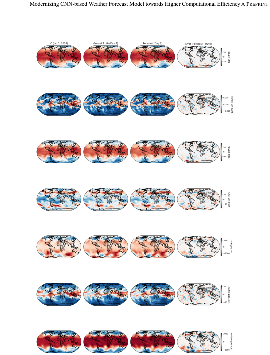
14 Modernizing CNN-based Weather Forecast Model towards Higher Computational EfficiencyA PREPRINT 5 Supplementary Materials We visualize forecasts produced by our model at lead times ranging from 1 day to 14 days for seven key atmospheric variables, including temperature, humi...
2018
-
[2016]
Aifs–ecmwf’s data-driven forecasting system
Simon Lang, Mihai Alexe, Matthew Chantry, Jesper Dramsch, Florian Pinault, Baudouin Raoult, Mariana CA Clare, Christian Lessig, Michael Maier-Gerber, Linus Magnusson, et al. Aifs–ecmwf’s data-driven forecasting system. arXiv preprint arXiv:2406.01465,
-
[2018]
Gaussian error linear units (gelus)
Dan Hendrycks and Kevin Gimpel. Gaussian error linear units (gelus). arXiv preprint arXiv:1606.08415,
-
[2020]
A historical, geographical and ecological perspective on the 2018 european summer drought,
Wouter Peters, Ana Bastos, Philippe Ciais, and Alex Vermeulen. A historical, geographical and ecological perspective on the 2018 european summer drought,
2018
-
[2021]
The extremely hot and dry 2018 summer in central and northern europe from a multi-faceted weather and climate perspective
Efi Rousi, Andreas H Fink, Lauren S Andersen, Florian N Becker, Goratz Beobide-Arsuaga, Marcus Breil, Giacomo Cozzi, Jens Heinke, Lisa Jach, Deborah Niermann, et al. The extremely hot and dry 2018 summer in central and northern europe from a multi-faceted weather and climate p...
2018
-
[2022]
Aardvark weather: end-to-end data-driven weather forecasting
Anna Vaughan, Stratis Markou, Will Tebbutt, James Requeima, Wessel P Bruinsma, Tom R Andersson, Michael Herzog, Nicholas D Lane, Matthew Chantry, J Scott Hosking, et al. Aardvark weather: end-to-end data-driven weather forecasting. arXiv preprint arXiv:2404.00411,
-
[2023]
Graphcast: Learning skillful medium-range global weather forecasting
Remi Lam, Alvaro Sanchez-Gonzalez, Matthew Willson, Peter Wirnsberger, Meire Fortunato, Ferran Alet, Suman Ravuri, Timo Ewalds, Zach Eaton-Rosen, Weihua Hu, et al. Graphcast: Learning skillful medium-range global weather forecasting. arXiv preprint arXiv:2212.12794,
-
[2024]
Fengwu: Pushing the skillful global medium-range weather forecast beyond 10 days lead
Kang Chen, Tao Han, Junchao Gong, Lei Bai, Fenghua Ling, Jing-Jia Luo, Xi Chen, Leiming Ma, Tianning Zhang, Rui Su, et al. Fengwu: Pushing the skillful global medium-range weather forecast beyond 10 days lead. arXiv preprint arXiv:2304.02948, 2023b. Junzhong Ji, Jing He, Mingl...
-
[2025]
The 2018 european heatwave led to stem dehydration but not to consistent growth reductions in forests
Roberto L Salomón, Richard L Peters, Roman Zweifel, Ute GW Sass-Klaassen, Annemiek I Stegehuis, Marko Smiljanic, Rafael Poyatos, Flurin Babst, Emil Cienciala, Patrick Fonti, et al. The 2018 european heatwave led to stem dehydration but not to consistent growth reductions in fo...
2018
Reviewed August 6, 2026 · model on record in the stance chip above.
Discussion (0). Sign in to comment.