REVIEW 3 major objections 5 minor 59 references
Dynamical analog spacetimes from nonlinear perturbations in a topological material
T0 review · 3 major / 5 minor · reviewed 2026-08-06 · deepseek-v4-flash
Pith's one-line read This paper claims that nonlinear density-wave perturbations in a topological-material electron fluid generate a time-dependent acoustic metric with an evolving horizon and a measurable microkelvin analog Hawking temperature.
desk verdict The nonlinear wave equation holds up, but the Hawking-temperature calculation is dimensionally wrong and off by orders of magnitude — the headline microkelvin claim is unsupported. read the letter →
The pith
A machine-rendered reading of the paper's core claim, the machinery that carries it, and where it could break.
The reading
What carries the argument
The central object is the nonlinear acoustic metric whose inverse components are $g^{tt}=A/(\rho r^2)$, $g^{tr}=F/(\rho r^2)$, and $g^{rr}=F^2/(\rho^3 r^6)-c_s^2/(A\rho r^2)$. It is generated by a perturbation variable $F=\rho v r^2/A$, which plays the role of a Berry-curvature-modified mass accretion rate; here $A$ is the Berry curvature correction, a quantum geometric phase effect on the electron's semiclassical motion. The wave equation $\partial_\mu(g^{\mu\nu}\partial_\nu F')=0$ carries all nonlinearities in the metric, and the horizon condition $g^{rr}=0$ locates the surface where the radial flow speed equals the local sound speed. This metric, together with the resulting surface gravity, is the machinery that turns electron-fluid perturbations into a laboratory analog of a black hole.
What would settle it
Recompute the second time derivative of the perturbed Euler equation while keeping every term for the exact background $v_0=b/r$ and the DFT density profile; if the omitted radial-derivative terms are nonzero at the claimed horizon $r_H=0.166614$ m, then the wave equation, the effective metric, and the reported $T_H\simeq9.99\,\mu\mathrm{K}$ must be revised.
Extended reading notes
Core claim
The paper's central claim is that all orders of a radial perturbation of a stationary, spherically symmetric, Berry-curvature-modified electron flow obey a single nonlinear wave equation $\partial_\mu(g^{\mu\nu}\partial_\nu F')=0$ for the variable $F=\rho v r^2/A$, where $A$ encodes the Berry correction. The inverse acoustic metric $g^{\mu\nu}$ depends on the full fluctuating density, velocity, and sound speed, so the geometry reacts to the perturbation as it propagates. The horizon sits where $g^{rr}=0$, equivalent to $|v|=c_s$, and expanding the metric around that radius gives a surface gravity $\kappa=\rho(r_H)b^2/(A r_H)$ for the velocity profile $v=b/r$, hence $T_H=\hbar\rho(r_H)b^2/(2\pi k_B A r_H)$. Using a DFT-derived graphene density and the parameters $b=-1999.37\ \mathrm{m^2/s}$, $c_s=12000\ \mathrm{m/s}$, $A=5$, the authors obtain $r_H\simeq0.166614$ m and $T_H\simeq9.99\times10^{-6}$ K. They further show numerically that first- and second-order perturbations localize near the horizon and, for low-frequency perturbations, drive the horizon to recede.
Load-bearing premise
The load-bearing premise is that the second time derivative of the perturbed Euler equation may be simplified by dropping all radial derivatives of the stationary background velocity and density, even though those derivatives do not vanish for the adopted $v_0=b/r$ background and the graphene density profile.
Editorial extensions
If this is right
- If the paper's central claim is correct, laboratory electron flows in graphene-like systems could exhibit analog Hawking temperatures of order ten microkelvin, within reach of existing low-temperature measurement techniques.
- The acoustic horizon becomes a dynamical object: high-frequency perturbations produce a horizon that relaxes toward its stationary location, while low-frequency perturbations make it recede.
- All nonlinear orders contribute to the effective metric, so the curvature of the emergent spacetime depends on the perturbation amplitude instead of being fixed by the background flow.
- The perturbation scheme yields a systematic order-by-order expansion of the metric corrections, so horizon formation and back-reaction can be tracked to arbitrary order in the accretion-rate variable.
Reading between the lines
- Editorial inference: the same accretion-rate perturbation variable could be used to engineer nonlinear analog horizons in other two-dimensional hydrodynamic systems, such as polariton condensates or cold-atom flows, where the density profile is created rather than computed ab initio.
- Editorial inference: the reported low-frequency receding horizon implies a concrete time-domain signature, a gradual inward drift of the surface where the flow speed equals the sound speed, that could be searched for in transport measurements of electron hydrodynamics.
- Editorial inference: the weakest step in the derivation could be tested directly by integrating the original nonlinear fluid equations numerically without the perturbative shortcut; discrepancies in horizon location or temperature would pinpoint exactly where the acoustic-metric reduction fails.
Editorial analysis
A structured set of objections, weighed in public.
Referee Report
Summary. The manuscript develops a nonlinear analog gravity framework for a Berry-curvature-modified electron fluid, using the mass-accretion-like variable F = ρ v r^2 / A. It derives an exact nonlinear wave equation for perturbations of F, packages it as propagation on a dynamical acoustic metric, expands the metric perturbatively to second order, and numerically studies horizon dynamics for a graphene-based model. The paper's advertised quantitative result is an analog Hawking temperature of roughly 10 microkelvin in experimentally accessible regimes.
Significance. The nonlinear wave-equation part of the paper is a genuine contribution if it stands: the derivation from the Euler equation is exact, the perturbative expansion of the acoustic metric to second order is systematic, and the idea of using a topological material as an analog spacetime platform is interesting. I want to be explicit that the reader's concern about the step from Eq. (9) to Eq. (10) does not land: for a barotropic fluid, time differentiation and spatial differentiation commute in the required way, so Eq. (10) is exact rather than an approximation. However, the central quantitative claim of the paper, the Hawking temperature, is undermined by a dimensional inconsistency and an arithmetic error in Eqs. (32), (33), and (38). Because that temperature is highlighted in the abstract and conclusion, the paper cannot be accepted in its current form.
major comments (3)
- [Sec. III, Eqs. (31)-(33)] The surface gravity κ defined in Eq. (31) and evaluated in Eq. (32) has incorrect dimensions. With ρ in C/m^2, b in m^2/s, and r_H in m, the combination κ = ρ(r_H) b^2 / (A r_H) has units C·m/s^2, not s^-1; if ρ were a conventional mass density, the units would be kg/s^2, again not s^-1. Consequently T_H = ℏκ/(2πk_B) in Eq. (33) does not have units of temperature. Even if the density factors were dimensionless, a 1/c_s factor would be needed to convert an acceleration into a rate before applying the Hawking formula. This is load-bearing because Eq. (33) is the basis for the abstract's claim of experimentally accessible microkelvin temperatures.
- [Sec. IV.D, Eq. (38)] The arithmetic in Eq. (38) is internally inconsistent. Substituting the stated values gives a quotient of order 10^17 K, not 9.98532 × 10^-6 K. The displayed microkelvin value is recovered only if the factor ℏ/k_B = 7.638226 × 10^-12 K s is moved from the denominator into the numerator, rather than appearing in the denominator as written. Thus the numerical Hawking-temperature claim of the abstract is not supported by the equations as written.
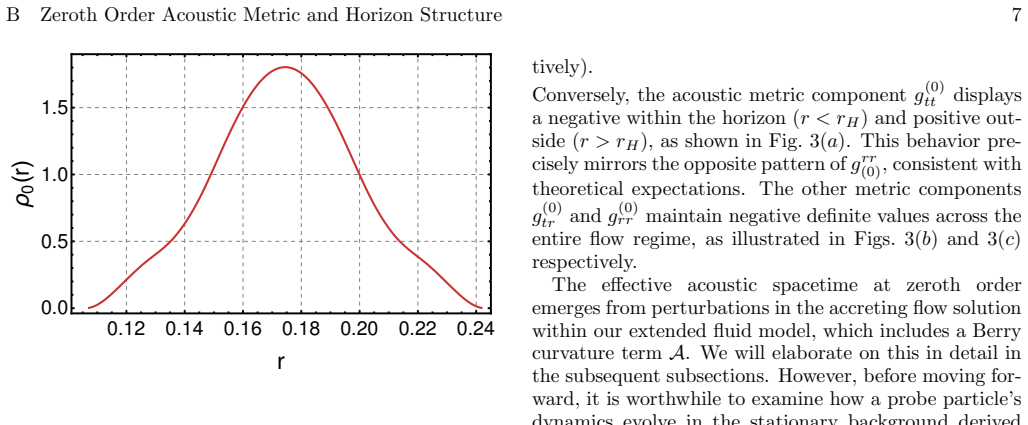
- [Sec. IV.A and Fig. 1] The background density profile is described as obtained from first-principles DFT, but the manuscript does not explain how a graphene unit-cell calculation yields the plotted macroscopic radial distribution with r in meters (0.1068 m to 0.2422 m), does not define the coordinate x in r ≡ √(2x), and does not give the fitting function or convergence details for the density profile. Since the value ρ(r_H) = 1.711766 C/m^2 is used in Eq. (38), the numerical results are not reproducible as reported.
minor comments (5)
- [Eq. (16)] In Eq. (16), the summation index is l but the expansion parameter is written as ϵ^k; this should be ϵ^l ζ_l(r,t).
- [Figs. 6-12 and text] Several figure cross-references are inconsistent: for example, the text describing Fig. 6 refers to Fig. 7 panels, and some captions cite the wrong equation numbers. The figures should be renumbered or the references corrected.
- [Sec. IV.A] The text says the radial coordinate is defined as r ≡ √(2x) but x is never introduced, and the mapping from a two-dimensional Cartesian coordinate to a radial variable in a spherically symmetric flow needs clarification.
- [Sec. IV.A] The DFT paragraph should specify the supercell geometry, k-point mesh used for the charge density, and the procedure by which the computed charge density is converted into the continuum profile ρ0(r) plotted in Fig. 1.
- [General] The manuscript contains numerous typographical and grammatical errors, including 'dimish', 'more amplified versions', and inconsistent use of 'the horizon position... are located'. An editorial pass is needed.
Circularity Check
No significant circularity: the nonlinear wave equation and Hawking temperature are derived from stated fluid equations and independently chosen parameters, with no fitted input renamed as a prediction.
full rationale
The derivation chain is self-contained in the sense relevant to circularity. The nonlinear wave equation, Eq. (11), and the inverse acoustic metric, Eq. (13), are obtained by substituting the perturbation decomposition (Eqs. (5)-(8)) and the continuity relation (Eq. (7)) into the time-differentiated Euler equation (Eqs. (9)-(10)); no parameter is fitted to the quantity being predicted, and the resulting wave equation is not equivalent by construction to its own ansatz. The Hawking temperature, Eq. (33), is evaluated in Eq. (38) from independently chosen parameters (b = -1999.37 m^2/s, c_s = 12000.0 m/s, A = 5) and the DFT-derived density rho(r_H) = 1.711766 C/m^2, rather than fitted to a target temperature. Whether the displayed arithmetic and dimensions in Eq. (38) are correct is a soundness issue, not a circularity issue. The self-citation to Ref. [26], authored by the corresponding author, supplies the starting Berry-curvature-modified fluid equations with stated semiclassical assumptions; those assumptions do not include the acoustic-metric or Hawking-temperature results, and the later derivation does not rely on Ref. [26] to establish those results. Refs. [17, 24, 25] are used as standard background formalism and benchmark behavior, not as a substitute for the derivation. No fitted input is renamed as a prediction, and no load-bearing argument reduces to a self-citation.
Assumptions & free parameters
free parameters (4)
- Berry curvature factor A =
5
- specific angular momentum b =
-1999.37 m^2/s
- sound speed c_s =
12000.0 m/s
- perturbation frequencies =
omega_high=10^6 rad/s, omega_low=10^4 rad/s
assumptions (5)
- domain assumption The Berry-curvature-modified fluid equations (Eqs. 1 and 2) from Ref. [26] correctly describe electron hydrodynamics in graphene.
- ad hoc to paper A = 1 + e(Omega.B) is a constant.
- ad hoc to paper The perturbed Euler equation can be time-differentiated to yield Eq. (10) with background gradient terms omitted.
- domain assumption The fluid flow is spherically symmetric with radial velocity v=b/r.
- standard math The two-dimensional metric can be promoted to 3+1 dimensions so that the scalar-field equation (14) holds.
Cite this review
Pith. "Pith review of Dynamical analog spacetimes from nonlinear perturbations in a topological material." pith.science (2026). https://pith.science/paper/MF5WADLG
@misc{pith2026250716570,
  author       = {Pith},
  title        = {Pith review of: Dynamical analog spacetimes from nonlinear perturbations in a topological material},
  year         = {2026},
  howpublished = {\url{https://pith.science/paper/MF5WADLG}},
  note         = {Machine review of arXiv:2507.16570}
}
read the original abstract
Emergent spacetime analogs in condensed matter systems have opened a fascinating window into simulating aspects of gravitational physics in controlled laboratory environments. In this work, we develop a comprehensive nonlinear analog gravity framework within a topological material, incorporating the impact of Berry curvature on the hydrodynamic flow of electrons. Unlike prevalent studies in existing literature limited to linear perturbations, we derive and analyze a fully nonlinear wave equation governing radial perturbations of density and velocity fields, which dynamically generate an effective acoustic metric. Taking the example of graphene as a representative system, and calculating its properties from first principles, we numerically demonstrate the formation of evolving acoustic horizons and quantify analog Hawking temperatures in experimentally accessible regimes. Our findings suggest that topological materials can serve as versatile platforms to probe rich gravitational phenomena, including horizon dynamics and quasi-thermal emission, beyond conventional linear approximations. This work lays the groundwork for exploring nonlinear emergent spacetime in a broad class of quantum materials, bridging condensed matter physics and gravitational analogs.
Figures


Figures from the paper (9 more)


Reference graph
Works this paper leans on
-
[1]
High frequency perturbations First, for the Berry curvature incorporated accretion rate perturbations, in solving Eq. (18), we assume the trial solution ofF 1(r, t) of the form: F1(r, t) =gω(r)e−iωt .(39) Therefore using Eq. (39), from Eq. (18) one can have the following differential equation ofg ω(r). grr (0) g′′ ω + grr (0) ′ g′ ω −ω 2gtt (0) gω −iω 2gt...
-
[2]
Low frequency perturbations We now examine low frequency perturbations that de- cay exponentially over time. For this purpose, we nu- merically solve Eq. 40 withω low = 10 4 rad/s over the time intervalt= 0 s tot= 30 s. The full real space- time solution for the Berry curvature induced accretion rate,F 1(r, t), is presented in Fig. 9(a). The solution dis-...
-
[3]
W. G. Unruh, Phys. Rev. Lett.46, 1351 (1981)
1981
-
[4]
L. P. Euv´ e, F. Michel, R. Parentani, T. G. Philbin, and G. Rousseaux, Phys. Rev. Lett.117, 121301 (2016), arXiv:1511.08145 [physics.flu-dyn]
work page Pith review arXiv 2016
-
[5]
Steinhauer, Nature Phys.12, 959 (2016), arXiv:1510.00621 [gr-qc]
J. Steinhauer, Nature Phys.12, 959 (2016), arXiv:1510.00621 [gr-qc]
arXiv 2016
-
[6]
J. R. Mu˜ noz de Nova, K. Golubkov, V. I. Kolobov, and J. Steinhauer, Nature569, 688 (2019), arXiv:1809.00913 [gr-qc]
arXiv 2019
-
[7]
Observation of Stimulated Hawking Radiation in Optics
J. Drori, Y. Rosenberg, D. Bermudez, Y. Silberberg, and U. Leonhardt, Phys. Rev. Lett.122, 010404 (2019), arXiv:1808.09244 [gr-qc]
work page Pith review arXiv 2019
-
[8]
Magnonic Analogue of Black/White Hole Horizon in Superfluid $^3$He-B
M. ˇCloveˇ cko, E. Gaˇ zo, M. Kupka, and P. Skyba, Phys. Rev. Lett.123, 161302 (2019), arXiv:1810.09890 [cond- mat.other]
work page Pith review arXiv 2019
Show all 59 references
-
[9]
Vocke, C
D. Vocke, C. Maitland, A. Prain, K. E. Wilson, F. Bian- calana, E. M. Wright, F. Marino, and D. Faccio, Optica 5, 1099 (2018)
2018
-
[10]
D. D. Solnyshkov, C. Leblanc, S. V. Koniakhin, O. Bleu, and G. Malpuech, Phys. Rev. B99, 214511 (2019), arXiv:1809.05386 [cond-mat.quant-gas]
2019 arXiv
-
[11]
Aguero-Santacruz and D
R. Aguero-Santacruz and D. Bermudez, Phil. Trans. Roy. Soc. Lond. A378, 20190223 (2020), arXiv:2002.07907 [gr-qc]
2020 arXiv
-
[12]
Petty and F
J. Petty and F. K¨onig, Phil. Trans. R. Soc. A378, 20190231 (2020)
2020
-
[13]
Leonhardt, Phil
U. Leonhardt, Phil. Trans. Roy. Soc. Lond. A378, 20190229 (2020), arXiv:2001.03943 [gr-qc]
2020 arXiv
-
[14]
M. J. Jacquet et al., Phil. Trans. Roy. Soc. Lond. A378, 20190225 (2020), arXiv:2002.00043 [cond-mat.quant- gas]
2020 arXiv
-
[15]
M. P. Blencowe and H. Wang, Phil. Trans. Roy. Soc. Lond. A378, 20190224 (2020), arXiv:2003.00382 [quant- ph]
2020 arXiv
-
[16]
Bera and S
A. Bera and S. Ghosh, Phys. Rev. D101, 105012 (2020), arXiv:2001.08467 [hep-th]
2020 arXiv
-
[17]
M. A. Anacleto, F. A. Brito, and E. Passos, Phys. Lett. A380, 1105 (2016), arXiv:1309.1486 [hep-th]
2016 arXiv
-
[18]
M. J. Jacquet, S. Weinfurtner, and F. K¨ onig, Phil. Trans. Roy. Soc. Lond. A378, 20190239 (2020), arXiv:2005.04027 [gr-qc]
2020 arXiv
-
[19]
Barcelo, S
C. Barcelo, S. Liberati, and M. Visser, Living Rev. Rel. 14, 3 (2011), arXiv:gr-qc/0505065
2011 arXiv
-
[20]
Torres, S
T. Torres, S. Patrick, M. Richartz, and S. Weinfurtner, Phys. Rev. Lett.125, 011301 (2020), arXiv:1811.07858 [gr-qc]
2020 arXiv
-
[21]
H. Liu, H. Guo, and R. Ling, Phys. Rev. D110, 024035 (2024), arXiv:2404.04982 [gr-qc]
2024 arXiv
-
[22]
Patrick and S
S. Patrick and S. Weinfurtner, Phys. Rev. D102, 084041 (2020), arXiv:2007.03769 [gr-qc]
2020 arXiv
-
[23]
Sen and A
S. Sen and A. K. Ray, Phys. Rev. D89, 063004 (2014), arXiv:1207.1070 [astro-ph.GA]
2014 arXiv
-
[24]
Albuquerque and S
S. Albuquerque and S. H. V¨ olkel, Phys. Rev. D111, 124020 (2025), arXiv:2501.09000 [gr-qc]
2025 arXiv
-
[25]
Malato Corrˆ ea, C
M. Malato Corrˆ ea, C. F. B. Macedo, R. Panosso Macedo, and L. A. Oliveira, Phys. Rev. D112, 024036 (2025), arXiv:2504.00107 [gr-qc]
2025 arXiv
-
[26]
Fernandes, S
K. Fernandes, S. Maity, and T. K. Das, Phys. Rev. D 106, 025020 (2022), arXiv:2106.07618 [gr-qc]
2022 arXiv
-
[27]
Fernandes, S
K. Fernandes, S. Maity, and T. Das, Phys. Rev. D106, L021701 (2022)
2022
-
[28]
A. K. Mitra and S. Ghosh, Phys. Rev. D106, L041702 (2022), arXiv:2111.00473 [hep-th]
2022 arXiv
-
[29]
Sundaram and Q
G. Sundaram and Q. Niu, Phys. Rev. B59, 14915 (1999), arXiv:cond-mat/9908003
1999 arXiv
-
[30]
Xiao, M.-C
D. Xiao, M.-C. Chang, and Q. Niu, Rev. Mod. Phys.82, 1959 (2010), arXiv:0907.2021 [cond-mat.mes-hall]
2010 arXiv
-
[31]
Nagaosa, J
N. Nagaosa, J. Sinova, S. Onoda, A. H. MacDonald, and N. P. Ong, Rev. Mod. Phys.82, 1539 (2010), arXiv:0904.4154 [cond-mat.mes-hall]
2010 arXiv
-
[32]
Abrikosov, Introduction to the Theory of Normal Metals (Academic Press, New York, 1972)
A. Abrikosov, Introduction to the Theory of Normal Metals (Academic Press, New York, 1972)
1972
-
[33]
F. D. M. Haldane, Phys. Rev. Lett.93, 206602 (2004), arXiv:cond-mat/0408417
2004 arXiv
-
[34]
H. B. Nielsen and M. Ninomiya, Physics Letters B130, 389 (1983)
1983
-
[35]
Bohm et al., The Geometric Phase in Quantum Systems (Springer-Verlag, Berlin and Heidelberg, 2003)
A. Bohm et al., The Geometric Phase in Quantum Systems (Springer-Verlag, Berlin and Heidelberg, 2003)
2003
-
[36]
Duval, Z
C. Duval, Z. Horvath, P. A. Horvathy, L. Martina, and P. Stichel, Mod. Phys. Lett. B20, 373 (2006), arXiv:cond-mat/0506051
2006 arXiv
-
[37]
Gosselin, A
P. Gosselin, A. Berard, and H. Mohrbach, Eur. Phys. J. B58, 137 (2007), arXiv:hep-th/0603192
2007 arXiv
-
[38]
Chang and Q
M.-C. Chang and Q. Niu, Phys. Rev. Lett.75, 1348 (1995), arXiv:cond-mat/9505021
1995 arXiv
-
[39]
S. K. Das, D. Roy, and S. Sengupta, Pramana8, 117 (1977)
1977
-
[40]
Slavchov and R
R. Slavchov and R. Tsekov, J. Chem. Phys.132, 084505 (2010)
2010
-
[41]
Polini and A
M. Polini and A. K. Geim, Phys. Today73, 28 (2020)
2020
-
[42]
Lucas and K
A. Lucas and K. C. Fong, J. Phys. Condens. Matter30, 053001 (2018), arXiv:1710.08425 [cond-mat.str-el]
2018 arXiv
-
[43]
Mackenzie, N
A. Mackenzie, N. Nandi, S. Khim, P. Kushwaha, P. Moll, and B. Schmidt, L. Barletti J. Math. Ind.6, 7 (2016)
2016
-
[44]
J. A. Petterson, J. Silk, and J. P. Ostriker, Mon. Not. R. Astron. Soc.191, 571 (1980). 18
1980
-
[45]
Theuns and M
T. Theuns and M. David, Astrophys. J.384, 587 (1992)
1992
-
[46]
Frank, A
J. Frank, A. King, and D. J. Raine, Accretion Power in Astrophysics: Third Edition (Cam- bridge University Press, Cambridge, England, 2002)
2002
-
[47]
Visser, Class
M. Visser, Class. Quant. Grav.15, 1767 (1998), arXiv:gr- qc/9712010
1998
-
[48]
Schutzhold and W
R. Schutzhold and W. G. Unruh, Phys. Rev. D66, 044019 (2002), arXiv:gr-qc/0205099
2002 arXiv
-
[49]
P. E. Bl¨ ochl, Phys. Rev. B50, 17953 (1994)
1994
-
[50]
Kresse and J
G. Kresse and J. Hafner, Phys. Rev. B47, 558 (1993)
1993
-
[51]
Kresse and J
G. Kresse and J. Furthm¨ uller, Phys. Rev. B54, 11169 (1996)
1996
-
[52]
J. P. Perdew, K. Burke, and M. Ernzerhof, Phys. Rev. Lett.77, 3865 (1996)
1996
-
[53]
Dalui, A
S. Dalui, A. K. Mitra, D. Mitra, and S. Ghosh, Phys. Rev. D109, 064055 (2024), arXiv:2402.15540 [gr-qc]
2024 arXiv
-
[54]
Dalui, B
S. Dalui, B. R. Majhi, and P. Mishra, Phys. Rev. D102, 044006 (2020), arXiv:1910.07989 [gr-qc]
2020 arXiv
-
[55]
Dalui and B
S. Dalui and B. R. Majhi, Phys. Rev. D102, 124047 (2020), arXiv:2007.14312 [gr-qc]
2020 arXiv
-
[56]
Dalui and B
S. Dalui and B. R. Majhi, Phys. Lett. B826, 136899 (2022), arXiv:2103.11613 [gr-qc]
2022 arXiv
-
[57]
Sarsby, N
M. Sarsby, N. Yurttag¨ ul, and A. Geresdi, Nature Com- munications11, 1492 (2020)
2020
-
[58]
J. M. Edge, Y. Kedem, U. Aschauer, N. A. Spaldin, and A. V. Balatsky, Phys. Rev. Lett.115, 247002 (2015)
2015
-
[59]
J. S. J. A. Petterson and J. P. Ostriker, Mon. Not. R. Astr. Soc.191, 571 (1980)
1980
Reviewed August 6, 2026 · model on record in the stance chip above.
Discussion (0). Sign in to comment.