REVIEW 4 major objections 6 minor 85 references
Spectral distribution of sparse Gaussian Ensembles of Real Asymmetric Matrices
T0 review · 4 major / 6 minor · reviewed 2026-08-06 · deepseek-v4-flash
Pith's one-line read Average spectra of sparse real asymmetric matrices are fixed by a single complexity parameter $Y$, so ensembles with different sparsity structures share identical spectral densities whenever $Y$ matches, with real Ginibre statistics as…
desk verdict Useful framework extension, but the central evolution equation is derived under constraints that force the matrix to be normal, which excludes the target sparse real-asymmetric ensembles. read the letter →
The pith
A machine-rendered reading of the paper's core claim, the machinery that carries it, and where it could break.
The reading
What carries the argument
The load-bearing object is the complexity-parameter mapping of eq. (7): $Y=t_1=(2/M)\sum_{m,n}q_{mn;1}\ln(y_{mn}/|\gamma-2y_{mn}|)+c_0$, a single functional of all entry variances chosen so that $\partial\rho_1/\partial Y = L\rho_1$, where $L=\sum_{k,l}\partial^2/\partial H_{kl}^2 + \gamma\sum_{k,l}(\partial/\partial H_{kl})H_{kl}$ is the diffusion generator in matrix space. This reduction collapses the many-parameter ensemble dynamics into a one-parameter evolution, and carrying it through the eigenvalue joint density yields the evolution equations (17) for the real-eigenvalue density and (33)–(36) for the complex-pair density. The real-axis equation reduces to a Dyson–Pastur form once the repulsion integral $s_1(e)/e$ is kept only in leading order, giving Gaussian then semicircle solutions; the complex-plane equation separates in $r$ and $\theta$ and, after dropping the real–complex repulsion terms $J_c$ and $J_d$, adopts the complex-matrix solutions of [68] built from confluent hypergeometric functions, with uniform limit inside $\sqrt{N}$.
What would settle it
Measure the ensemble-averaged complex-plane density near the real axis for a small real-asymmetric sparse ensemble ($N\sim 10$–$20$, where the fraction of real eigenvalues is largest) and compare it with the complex-matrix solution of [68] that the paper adopts; a density excess near the real axis growing with the fraction of real eigenvalues would show the dropped terms $J_c$ and $J_d$ are not negligible. A second check: build two ensembles with identical $Y-Y_0$ but different variance profiles and compare their two-point correlation $R_{2z}$ — the paper's claim fixes only one-point densities, so any mismatch delineates the extent of the asserted universality.
Extended reading notes
Core claim
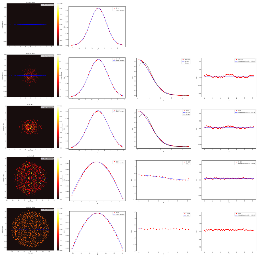
The paper's central claim is that the spectral joint probability density of a multiparametric Gaussian ensemble of real asymmetric matrices, with ensemble density $\rho(H;y,x)=\exp[-\sum_{k,l}(y_{kl}H_{kl}^{2}+x_{kl}H_{kl}H_{lk})]$, evolves in the complexity parameter $Y$ through $\partial P_1/\partial Y = (L_e + L_z)P_1$ (eq. (10)), so that the ensemble-averaged densities of real eigenvalues and of complex-conjugate pairs depend on the ensemble only through $Y-Y_0$. In the equilibrium limit the complex-plane density becomes constant inside a circle of radius $\sqrt{N}$, decays exponentially beyond it, and is independent of angle — the real Ginibre statistics — while the projected real-axis density runs from a Gaussian (small $Y-Y_0$) to a semicircle (large $Y-Y_0$). Numerical diagonalization of three sparse ensembles with different variance profiles (constant, power-law, and exponential off-diagonal decay) shows the density curves collapse when plotted against $Y$, confirming single-parameter control of the spectrum.
Load-bearing premise
The complex-plane density rests on three approximations the paper states explicitly: the real–complex repulsion terms $J_c$ and $J_d$ are dropped, pair correlations are factorized as products of one-point densities, and the complex density is taken as nearly angle-independent; if any of these fails, the predicted complex-plane density is the complex-matrix one rather than the real-asymmetric one.
Editorial extensions
If this is right
- For any Gaussian real-asymmetric ensemble — sparse, banded, or full — the average real and complex spectral densities are fixed by the single scalar $Y-Y_0$, so computing $Y$ from the entry variances predicts the spectrum without large-scale diagonalization.
- The real-eigenvalue density crosses from a Gaussian to a semicircle as $Y-Y_0$ grows, while the complex-pair density flattens to uniformity inside radius $\sqrt{N}$ with exponential decay outside, recovering the real Ginibre steady state in the $Y\to\infty$ limit.
- Ensembles with equal $Y-Y_0$ and equal initial statistics share identical spectral densities even away from equilibrium, so the Poisson-to-Ginibre crossover has a universal shape across sparsity structures, not just a universal endpoint.
- The same complexity-parameter evolution extends to correlated, non-zero-mean ensembles of the form (1), as the numerical multivariate case indicates, although the explicit $Y$ for that case is not yet derived.
Reading between the lines
- The universality established here concerns one-point densities; whether two-point correlations (the level-repulsion profile) also collapse under $Y$ is untested, and a mismatch there would bound the universality claim rather than break it.
- Because the complex-plane equation is inherited from the complex-matrix case by dropping the real–complex repulsion, the regime where real eigenvalues are abundant — small $N$ or strongly banded matrices — is the natural place to look for deviations, and the paper's numerics do not resolve that regime.
- For neural-network practice the paper suggests a cheap diagnostic it does not itself propose: track the complexity parameter $Y$ of the weight matrix during training, since the spectral edge (and hence stability of the silent state) is governed by it.
Editorial analysis
A structured set of objections, weighed in public.
Referee Report
Summary. The paper claims to extend the complexity-parameter (Y) framework to sparse Gaussian ensembles of real asymmetric matrices. It derives (with details deferred to supplemental material) an evolution equation for the spectral joint probability density function, solves approximate equations for the real-eigenvalue density and the complex-eigenvalue density, and confronts these with exact diagonalization of four ensembles (BE, PE, EE, ME). The authors conclude that the spectral statistics depend on the ensemble only through Y, revealing a universality across sparse structures.
Significance. The target class of sparse real asymmetric matrices is highly relevant to neuroscience and machine learning, and a one-parameter description of their spectral densities would be a valuable theoretical tool. The paper's numerical data (Fig. 1) show a suggestive collapse of the real-to-complex eigenvalue ratio as a function of Y. However, the central derivation is not verifiable from the main text, the key eigenvector conditions are incompatible with non-normal matrices, and the quantitative comparisons rely on per-ensemble fits. As a result, the paper does not provide a trustworthy derivation or a falsifiable predictive test. The absence of machine-checked proofs or reproducible code further limits the assessment to the analytic arguments and the reported fits.
major comments (4)
- [Section II.B, Eqs. (10)-(12)] The derivation of the spectral JPDF uses U V = I together with U U^T = I and V V^T = I. For E = U H V with U V = I, these conditions force V = U^T and H = U^T E U, hence H H^T = H^T H, i.e., H is normal. The target ensembles BE, PE, EE, and ME consist of generic non-normal real matrices, so this derivation cannot be applied to them. The paper's own remarks in Section II.B, noting that different eigenvector conditions in [46] and [68] lead to different eigenvalue dynamics, indicate that the normalization is consequential rather than a harmless gauge choice. Therefore Eq. (10) is not established for the class of matrices under study, and the solutions in Sections III and IV inherit this gap.
- [Section VI, Eqs. (43)-(44) and Table I] The 'agreement with theory' is largely a fitting exercise. The initial density R1(r; Y0) is obtained by numerical fit, the coefficients q_1nu and chi in Eqs. (43)-(44) are determined by numerical fits for each ensemble and b value, and the real-line densities are fitted with Gaussian parameters C1 and q that vary with b. No cross-prediction is made: ensembles at the same (Y-Y0) are not compared with one another using common parameters. The collapse in Fig. 1 concerns a single scalar ratio, not the full spectral density. Thus the numerical results provide only weak, non-falsifiable support for the complexity-parameter universality claim.
- [Section IV.B, after Eq. (42)] The neglect of the real-complex repulsion terms J_c and J_d is asserted without quantitative justification; the statement that they are 'relatively smaller' than I_c and I_d is not demonstrated. For small b, a substantial fraction of eigenvalues are real (Fig. 1), so the real-complex interaction may be non-negligible. Since the complex-plane solution is then taken verbatim from the complex-matrix case [68], the derived R1z is not shown to be the density of the real-asymmetric ensemble. The weak theta-dependence of R1z is also inferred from the same numerical data that are subsequently fitted, making the argument circular.
- [Sections II.B and IV.B; Supplemental Material [83]] The central derivation of Eq. (10) and the detailed solution of the complex-plane equation are deferred to supplemental material [83], which is not included for review. Given that the validity of Eq. (10) is contested above, the omission of this material prevents verification of the load-bearing steps, including the response of eigenvalues and eigenvectors to matrix perturbations. For a paper whose quantitative predictions rest on this equation, the main text should contain enough detail for the derivation to be checked.
minor comments (6)
- [Section V] The paragraph beginning 'Based on the analysis discussed in previous section...' is an exact duplicate of the preceding paragraph and should be removed.
- [Tables] Both the real-line fit table and the complex-plane fit table are labeled 'TABLE I'; they should be renumbered as Tables I and II, and the in-text references updated accordingly.
- [Throughout] There are several typos: 'exhibitory' should be 'excitatory' (Abstract), 'assymetric' appears in Section VII, and reference [73] is garbled ('Paslur L A 1972 Th. Math. Phyx. IO 67' should be 'Pastur L A 1972 Theor. Math. Phys. 10 67').
- [Fig. 5 caption] The caption says 'The other details of the figure are same as in figure 2' but also states the figure is for EE; the figure is actually for the multivariate (ME) case, so the caption should be corrected.
- [Table I (complex-plane fits)] The fit labels 'fita1, fitb1, fitn' are not defined in the main text; the functional forms should be defined or explicitly referenced to the supplemental material.
- [Introduction / Notation] The notation warning that subscripts change meaning is helpful, but the paper would benefit from a consolidated notation table to reduce ambiguity in equations such as (7), (21), and (43).
Circularity Check
Spectral-density 'predictions' reduce to fitted initial densities and fitted mode coefficients; the complex-plane result is also imported from same-author prior work.
-
fitted input called prediction
[Section VI, complex-plane analysis, around Eqs. (43)-(44) and Table I]
"As our formulation is based on a prior knowledge of initial density R 1(r, θ;Y0), we determine it by a numerical fit. The latter gives, for the initial ensemble at b=b 0 = 1/N, R 1(r, θ;Y0)≡R 1(r;Y 0) =A r −1/2 J1/2(Br) e −Cr 2 with A, B, Cas constants (the values for each ensemble given in table I). ... with only first few terms (withν≤2) retained in the P ν and the constantsq 1ν ofU 1ν determined by numerical fits; the fitting parameters in each case are given in table I."
Equation (43) is an eigenmode expansion of the initial density; the coefficients q_{1ν} are not derived from Y0 or from the complexity parameter, but fitted to the same radial density curves that the equation is claimed to predict. Since the initial A, B, C are also fitted at b=1/N and q_{1ν} are refitted for each b, the 'agreement' between eq. (43) and Figs. 2-4 is a multi-parameter curve fit, not an independent prediction of the complexity-parameter evolution.
-
fitted input called prediction
[Section III.B and Section VI, real-line fits; Eqs. (24)-(27) and Table I]
"As an example, we determine R 1(e, Y) from eq.(24) for a Gaussian initial level-density R1(e;Y 0) = 1√ 2πσ2 e− x2 2σ2 ; (this is the case analyzed later in our numerical analysis too discussed in section VI). ... the numerically fitted functions; the latter in each case agrees with our theoretical prediction i.e a Gaussian for small Y−Y 0 and a semicircle for large Y−Y 0."
The Gaussian shape is inserted as the assumed initial condition, and Table I Fit 1 refits C1 and q at every b value (e.g. C1=0.317, q=0.315 at b=1/N; different values at 1.5, 2.5, 15 and N). The theoretical solution (27) is not used to predict those parameters from Y−Y0; instead the same Gaussian functional form is fitted to each dataset and then labelled as agreement with theory. This is the fitted initial condition renamed as a prediction.
1 more flagged steps
-
other
[Section III.B, after Eq. (20), truncation of I_ez]
"Based on insights given by our numerical analysis for three prototypical cases of the ensemble (2) (discussed later in section VII), R 1z(r, θ) does not vary significantly with θ. This along with cos(mθ) present in both s m and l m implies a faster oscillation of integrand as m increases."
The weak θ-dependence of R1z used to truncate the series to m=1 is inferred from the same numerical data that later serve as the target of the theoretical fit. The simplified evolution equation (22) is therefore calibrated on the data it is then said to predict. This does not make the full derivation circular, but it weakens the numerical confirmation of the complexity-parameter universality.
full rationale
The paper does derive an evolution equation (10) for the spectral JPDF from the ensemble density, so the central formalism is not circular by construction. However, the numerical validation presented as 'agreement with our theoretical prediction' is substantially circular: the complex-plane density is expanded in modes whose coefficients q_{1ν} are fitted to the data, and the initial density is also obtained by a numerical fit; the real-line Gaussian shape is inserted as the initial condition and then refitted at every b. The weak θ-dependence that justifies truncating the series is itself inferred from the same data. These are fitted inputs called predictions. We do not count the reliance on [68] as circular because it is a published prior derivation by the same group, though it means the complex-plane solution is not independently re-derived here. Separately, the orthogonality condition U U^T=I, V V^T=I imposed in Section II.B would force normal matrices, which is a serious correctness concern for non-normal sparse real-asymmetric ensembles, but it is not a circularity of the type scored here. Overall, the core equations are independent, but the paper's claimed numerical confirmations of the spectral-density predictions reduce in part to curve fitting, giving a score of 6.
Assumptions & free parameters
free parameters (5)
- gamma =
1
- Initial complex density constants A, B, C =
A=1.06, B=0.73, C=0.294 for BE (Table I)
- Fitting coefficients q_1nu =
For BE: q_10=1.151, q_11=-4.333, q_12=108.132 (Table I)
- chi =
0.088
- Real-density Gaussian parameters C1, q =
For BE at b=1/N: C1=0.317, q=0.315 (Table I)
assumptions (5)
- domain assumption The ensemble density in eq. (2) admits a complexity parameter mapping in which the evolution is governed by a single parameter t1 = Y
- domain assumption The real asymmetric matrix is diagonalizable with U U^T = I and V V^T = I, with no exceptional points
- domain assumption Two-point spectral correlations factorize, R2 ~ R1 R1, for distances beyond the mean level spacing
- ad hoc to paper R1z(r,theta) has weak theta-dependence, so the m >= 1 terms in eq. (21) are negligible
- ad hoc to paper The real-complex eigenvalue repulsion terms J_c and J_d are negligible compared with I_c and I_d
invented entities (1)
-
Complexity parameter Y and complexity constants t_alpha
Cite this review
Pith. "Pith review of Spectral distribution of sparse Gaussian Ensembles of Real Asymmetric Matrices." pith.science (2026). https://pith.science/paper/6UIVQZ3Y
@misc{pith2026250721002,
  author       = {Pith},
  title        = {Pith review of: Spectral distribution of sparse Gaussian Ensembles of Real Asymmetric Matrices},
  year         = {2026},
  howpublished = {\url{https://pith.science/paper/6UIVQZ3Y}},
  note         = {Machine review of arXiv:2507.21002}
}
read the original abstract
Theoretical analysis of biological and artificial neural networks e.g. modelling of synaptic or weight matrices necessitate consideration of the generic real-asymmetric matrix ensembles, those with varying order of matrix elements e.g. a sparse structure or a banded structure. We pursue the complexity parameter approach to analyze the spectral statistics of the multiparametric Gaussian ensembles of real asymmetric matrices and derive the ensemble averaged spectral densities for real as well as complex eigenvalues. Considerations of the matrix elements with arbitrary choice of mean and variances render us the freedom to model the desired sparsity in the ensemble. Our formulation provides a common mathematical formulation of the spectral statistics for a wide range of sparse real-asymmetric ensembles and also reveals, thereby, a deep rooted universality among them.
Figures


Figures from the paper (2 more)

Reference graph
Works this paper leans on
-
[46]
J.T.Chalker and Z.J.Wang, Phys. Rev. Lett. 79, 1797, (1997)
work page 1997
-
[68]
however focussed on the spectral density analysis only for the complex matrices. With real random matrices appearing more often among complex systems studies, a derivation of their spectral density is desirable too.With present study focused on the real asymmetric matrices, we briefly review, in sections II.A and II.B, the complexity parameter formulation...
- [83]
-
[1]
Crisanti, H
H.J.Sommers, A. Crisanti, H. Sompolinsky and Y. Stein, Phys. Rev. Lett., 60, 1895 (1988)
1988
-
[2]
For small (Y−Y 0), therefore,⟨R 1(r, θ, Y)⟩θ remains almost of the same form as the initial density except for a change of coefficients
and also in supplemental material [83], this leads to ⟨R1(r, θ, Y)⟩θ = ∞X ν=0 U1ν e−νϕ ≈ ⟨R1(r, θ, Y0)⟩θ −ϕ ∞X ν=1 ν U1ν (43) 22 withU 10 =⟨R 1(r, θ, Y0)⟩θ andU 1ν ≡q 1ν F1 νχ+ 1, 3 2 ,− γr 2 2 forν >0 (see details in [83]). For small (Y−Y 0), therefore,⟨R 1(r, θ, Y)⟩θ remains almost of the same form as the initial density except for a change of coefficie...
-
[3]
Ranjan and L
K. Ranjan and L. F. Abbott, Phys. Rev. Lett., 97, 188104, (2006)
2006
-
[4]
D.R.Nelson and N.M.Shnerb, 58, 1383, (1998)
1998
-
[5]
Y. Ahmadian, F. Mumarola and K. D. Miller, Phys. Rev. E 91, 012820, (2015)
work page 2015
Show all 85 references
-
[6]
A. Amir, N. Hatano and D. R. Nelson, Phys. Rev. E 93, 042310, (2016)
2016
-
[7]
Granziol, S
D. Granziol, S. Zohren and S. Roberts, Learning Rates as a Function of Batch Size: A Random Matrix Theory Approach to Neural Network Training, Journal of Machine Learning Research 23 (2022) 1-65
2022
-
[8]
Pastur, On random matrices arising in deep neural networks: Gaussian case, Pure Appl
L. Pastur, On random matrices arising in deep neural networks: Gaussian case, Pure Appl. Funct. Anal. (2020), in press, arXiv:2001.06188
2020 arXiv
-
[9]
Pennington and P
J. Pennington and P. Worah, Nonlinear random matrix theory for deep learning, Journal of Statistical Mechanics: Theory and Experiment, 2019(12):124005, dec 2019. doi: 10.1088/1742- 5468/ab3bc3
2019 doi
-
[10]
Pennington and Y
J. Pennington and Y. Bahri, Geometry of Neural Network Loss Surfaces via Random Matrix Theory, Proceedings of the 34 th International Conference on Machine Learning, Sydney, Australia, PMLR 70, 2017
2017
-
[11]
Thamm, M
M. Thamm, M. Staats and B. Rosenow, Random matrix analysis of deep neural network weight matrices, Physical Review E, 106(5):054124, 2022
2022
-
[12]
Ghorbani, S
B. Ghorbani, S. Krishnan, and Y. Xiao, An investigation into neural net optimization via Hessian eigenvalue density. arXiv preprint arXiv:1901.10159, 2019
1901 arXiv
-
[13]
A. K. Lampinen and S. Ganguli, An analytic theory of generalization dynamics and transfer learning in deep linear networks. preprint arXiv:1809.10374, 2018
2018 arXiv
-
[14]
Louart, Z
C. Louart, Z. Liao, and R. Couillet. A random matrix approach to neural networks. The Annals of Applied Probability, 28(2):1190 – 1248, 2018. doi: 10.1214/ 17-AAP1328. 27
2018
-
[15]
Pennington, S
J. Pennington, S. Schoenholz and S. Ganguli, The emergence of spectral universality in deep networks, Proc. Mach. Learn. Res. 84 (2018) 1924–1932, arXiv:1802.09979
2018 arXiv
-
[16]
Seroussi and Z
I. Seroussi and Z. Ringel. Separation of scales and a thermodynamic description of feature learning in some cnns. preprint arXiv:2112.15383, 2021
2021 arXiv
-
[17]
preprint arXiv:2006.07721, 2020
Diego Granziol, Beyond random matrix theory for deep networks. preprint arXiv:2006.07721, 2020
2006 arXiv
-
[18]
N. P. Baskerville, D. Granziol, and J. P. Keating. Applicability of Random Matrix Theory in Deep Learning. preprint arXiv:2102.06740
-
[19]
Martin, T (Serena) Peng, and M
C H. Martin, T (Serena) Peng, and M. W. Mahoney. Predicting trends in the quality of state- of-the-art neural networks without access to training or testing data. Nature Communications, 12(1):4122, 2021. doi: 10.1038/s41467-021-24025-8
2021 doi
-
[20]
Implicit self-regularization in deep neural networks: Evi- dence from random matrix theory and implications for learning
C H Martin and M W Mahoney. Implicit self-regularization in deep neural networks: Evi- dence from random matrix theory and implications for learning. Journal of Machine Learning Research, 22(165):1–73, 2021
2021
-
[21]
Okuma, K
N. Okuma, K. Kawabata, K. Shiozaki, and M. Sato, Phys.Rev. Lett.124, 086801 (2020)
2020
-
[22]
D. S. Borgnia, A. J. Kruchkov, and R.-J. Slager, , Phys. Rev.Lett.124, 056802 (2020)
2020
-
[23]
M. S. Rudner and L. S. Levitov, Phys. Rev. Lett.102,065703 (2009)
2009
-
[24]
Yao and Z
S. Yao and Z. Wang, Phys. Rev. Lett.121,086803 (2018)
2018
-
[25]
Esaki, M
K. Esaki, M. Sato, K. Hasebe, and M. Kohmoto, Phys. Rev. B84, 205128 (2011)
2011
-
[26]
Y. C. Hu and T. L. Hughes, Phys. Rev. B84, 153101 (2011)
2011
-
[27]
Schomerus, Opt
H. Schomerus, Opt. Lett.38, 1912 (2013)
2013
-
[28]
Z. Gong, Y. Ashida, K. Kawabata, K. Takasan, S. Hi-gashikawa, and M. Ueda, Phys. Rev. X8, 031079 (2018)
2018
-
[29]
N.Moiseyev, Non-Hermitian Quantum Mechanics (Cambridge University Press, 2011)
2011
-
[30]
Ashida, Z
Y. Ashida, Z. Gong, and M. Ueda, Advances in Physics 69, 249 (2020)
2020
-
[31]
Zabalo, M
A. Zabalo, M. J. Gullans, J. H. Wilson, R. Vasseur,A. W. W. Ludwig, S. Gopalakrishnan, D. A. Huse, and J. H. Pixley, Phys. Rev.Lett. 128, 050602 (2022)
2022
-
[32]
Skinner, J
B. Skinner, J. Ruhman, and A. Nahum, Phys. Rev. X9, 031009 (2019)
2019
-
[33]
Feinberg and A
J. Feinberg and A. Zee, Phys. Rev. E59, 6433 (1999)
1999
-
[34]
A. C. Potter and R. Vasseur, arXiv e-prints, arXiv:2111.08018 (2021), arXiv:2111.08018 28
2021 arXiv
-
[35]
Huang and B
Y. Huang and B. I. Shklovskii, Phys. Rev. B 101, 014204 (2020)
2020
-
[36]
L. G. Molinari, Journal of Physics A: Mathematical and Theoretical 42, 265204 (2009)
2009
-
[37]
G. L. Celardo, M. Angeli, and R. Kaiser, arXiv preprint arXiv:1702.04506 (2017)
2017 arXiv
-
[38]
Kawabata and S
K. Kawabata and S. Ryu, Phys. Rev. Lett.126, 166801(2021)
2021
-
[39]
C. E. Maximo, N. A. Moreira, R. Kaiser, and R. Bachelard, Phys. Rev. A100, 063845 (2019)
2019
-
[40]
Cottier, A
F. Cottier, A. Cipris, R. Bachelard, and R. Kaiser, Phys. Rev. Lett.123, 083401 (2019)
2019
-
[41]
Hatano and D.R.Nelson, Phys
N. Hatano and D.R.Nelson, Phys. Rev. Lett. 77, 570 (1996); K.B. Efetov, Phys Rev. B 56 9630 (1997); I.Y. Glodsheild and B.A. Khoruzhenko, Phys. Rev. Lett., 80, 2897 (1998); C.Mudry, B.D.Simons and A.Altland, Phys. Rev. Lett., 80, 4257 (1998)
1996
-
[42]
A. Guo, G. J. Salamo, D. Duchesne, R. Morandotti, M. Volatier-Ravat, V. Aimez, G. A. Siviloglou, and D. N.Christodoulides, Phys. Rev. Lett.103,093902 (2009)
2009
-
[43]
M. L. Mehta, Random Matrices (Academic, New York, 1991)
1991
-
[44]
Haake, Quantum Signatures of Chaos (Springer-Verlag, Berlin, 1991)
F. Haake, Quantum Signatures of Chaos (Springer-Verlag, Berlin, 1991)
1991
-
[45]
J.T.Chalker and B.Mehlig, Phys. Rev. Lett. 81, 3367, (1998)
1998
-
[47]
Ginibre, J
J. Ginibre, J. Math. Phys. 6 440, (1965)
1965
-
[48]
Shukla, Phys
P. Shukla, Phys. Rev. Lett. 87, 19, 194102, (2001)
2001
-
[49]
Nils Lehmann and H-j Sommers, Phys. Rev. Lett. 67, 941, (1991)
1991
-
[50]
B, 88, 359, (1992)
F.Haake et al., Z.Phys. B, 88, 359, (1992)
1992
-
[51]
Bender and S
C.M. Bender and S. Boettcher, Phys. Rev. Lett. 80, 5243, (1998)
1998
-
[52]
Bender, N
C.M. Bender, N. Hassanpour, D.W.Hook, S.P.Klevansky, C. Sunderhauf and Z. Wen, Phys. Rev. A 95, (2017)
2017
-
[53]
Mostafazadeh, J
A. Mostafazadeh, J. Math. Phys. 43, 205, (2002); 43, 2814, (2002); 43, 3944, (2002)
2002
-
[54]
Bender, D.C
C.M. Bender, D.C. Brody and H.F.Jones, Phys. Rev. Lett. 89, (2002)
2002
-
[55]
Mudute-Ndumbe and M
E-M Graefe, S. Mudute-Ndumbe and M. Taylor, J. Phys. A: Math. Theo. 48, 38FT02, (2015)
2015
-
[56]
karr, Phys
Y.N.Joglekar and W.A. karr, Phys. Rev. E, 83, (2011)
2011
- [57]
-
[58]
Rotter, J
I. Rotter, J. Phys. A: Math. Theo., 42, 153001, (2009)
2009
-
[59]
Sommers, Phys
Y.V.Fyodorov, B.A.Khoruzhenko and H.-J. Sommers, Phys. Rev. Lett., 79, 557, (1997). 29
1997
-
[60]
Sommers, J
Y.V.Fyodorov and H.-J. Sommers, J. Math. Physics (N.Y.), 38, 1918, (1997)
1997
-
[61]
Feinberg and A.Zee, Phys
J. Feinberg and A.Zee, Phys. Rev. E 59, 6433, (1999)
1999
-
[62]
Y.V.Fyodorov and B.A.Khoruzhenko, Ann. Inst. Henri Poincare (Physique Theorique), 68, 449, (1998)
1998
-
[63]
Hamazaki, K
R. Hamazaki, K. Kawabata, N. Kura and M. Ueda, Phys. Rev. Res., 2, 023286, (2020)
2020
-
[64]
L. Sa, P. Ribciro and T. Prosen, Phys. Rev. X, 10, 021019, (2020)
2020
-
[65]
Bohigas and M
O. Bohigas and M. P. Pato, J. Phys. A: Math. Theor. 46, 115001, (2013)
2013
-
[66]
Khaymovich, Phys
G.De Tomasi and I. Khaymovich, Phys. Rev. B, 106, 094204 (2022)
2022
-
[67]
Suthar, Y-C Wang, Y-P Huang, H.H.Jens and J-H You, Phys
K. Suthar, Y-C Wang, Y-P Huang, H.H.Jens and J-H You, Phys. Rev. B 106, 064208 (2022)
2022
-
[69]
A. M. Garcia-Garicia, S. M. Nishigaki and J.J.M. Verbaarschot, Phys. Rev. E 66, 016132, (2002)
2002
-
[70]
Anasari and P
M.G. Anasari and P. Shukla, J. Phys. A: Math. Theor. (IOP), 57, 095005, (2024)
2024
-
[71]
Anasari and P
M.G. Anasari and P. Shukla, J. Phys. A: Math. Theor. (IOP) 57 455001, (2024)
2024
-
[72]
A. M. Mambuca, C. Cammarota and I. Neri, Phys. Rev. E 105, 014305 (2022)
2022
-
[73]
Neri and F
I. Neri and F. Lucas Metz, Phys. Rev. Research, 2, 033313 (2020)
2020
-
[74]
Shukla, Int
P. Shukla, Int. Jou. of Mod.Phys B (WSPC), 26, 12300008, (2012)
2012
-
[75]
Paslur L A 1972 Th. Math. Phyx. IO 67
1972
-
[76]
Kumar and A.Pandey, Annals of Physics
S. Kumar and A.Pandey, Annals of Physics
-
[77]
Pandey, Phase Transitions (Taylor and Francis), 77, 835 (2004)
A. Pandey, Phase Transitions (Taylor and Francis), 77, 835 (2004)
2004
-
[78]
Shukla, Phys
P. Shukla, Phys. Rev. B, 98, 054206 (2018)
2018
-
[79]
Neri and T
F.L.Metz, I. Neri and T. Rogers, J. Phys. A: Math. Theor. 52, 434003, (2019)
2019
-
[80]
I. I. Arkhipov and F. Minganti, Phys. Rev. A, 107, 012202 (2023)
2023
-
[81]
A.Pandey and P.Shukla, J. Phys. A, (1991)
1991
-
[82]
Temme and E.J.M
N.M. Temme and E.J.M. Veling, Indagationes Mathematicae (Elsevier) 33, 1221, (2022)
2022
-
[84]
Megginson,An introduction to Banach Space theory, Springer, N.Y
R.E. Megginson,An introduction to Banach Space theory, Springer, N.Y. (1998)
1998
-
[85]
Supplemental material. 30 FIG. 1.Ratio of the real eigenvalues and complex conjugate pairs:The figure displays the ratioL/MofLreal eigenvalues andMcomplex conjugate pairs for manybvalues and fixed N= 1024 for three ensembles withN=L+ 2M. As clear from the figure, the number of...
Reviewed August 6, 2026 · model on record in the stance chip above.
Discussion (0). Continue with ORCID to comment.