REVIEW 4 major objections 6 minor 45 references
Wavelets for power spectral density estimation of gravitational wave data
T0 review · 4 major / 6 minor · reviewed 2026-08-05 · deepseek-v4-flash
Pith's one-line read Wavelet smoothing of the log-periodogram yields gravitational-wave noise PSDs with high frequency resolution and low variance at once, beating the Welch PSD; for non-stationary noise, a median WDM wavelet-packet PSD is more robust.
desk verdict A competent application of known wavelet denoising to GW PSD estimation, with a clever variance-matching threshold, but the performance claims rest on a single event and a significance level tuned on the same data. read the letter →
The pith
A machine-rendered reading of the paper's core claim, the machinery that carries it, and where it could break.
The reading
What carries the argument
The load-bearing object is the log-periodogram identity $\ln P_{xx}(f)+\gamma=\ln S_{xx}(f)+\epsilon(f)$, with $\gamma$ the Euler–Mascheroni constant and $\mathrm{Var}[\epsilon]=\pi^2/6$. A discrete wavelet transform decomposes the left side into detail and approximation coefficients; percentile soft thresholding under a generalized Gaussian model removes the $\epsilon$ fluctuation from each detail level, and the inverse transform reconstructs $\ln S_{xx}(f)$. For non-stationary noise, the machinery is the wavelet packet transform read as an evolutionary power spectrum: taking the median across time of the squared coefficients in each frequency band yields the median wavelet packet PSD, and
What would settle it
Take simulated stationary noise with a known PSD containing a narrow line; compute wavelet smoothing PSDs over many realizations. If, with $s$ chosen so $\mathrm{Var}[\epsilon]\approx\pi^2/6$, the line's width is broadened or the residual noise variance does not approach $\pi^2/6$ without bias, the central denoising claim fails.
Extended reading notes
Core claim
The paper's central discovery is that a periodogram can be denoised instead of averaged: after $\ln P_{xx}(f)+\gamma=\ln S_{xx}(f)+\epsilon(f)$, the fluctuation term is Gumbel with variance $\pi^2/6$, so wavelet thresholding of detail coefficients removes $\epsilon(f)$ while preserving resolution. On GW150914 H1 data, wavelet smoothing achieves quality factor $Q=0.001528$ versus $0.001353$, matched-filter SNR $19.38$ versus $19.27$, and on 128 s of off-source data a Bayes factor $311.71$ versus $285.50$ when compared with Welch. For non-stationary noise, a median wavelet-packet PSD—especially the median WDM PSD—is more robust than the median periodogram at lines near 60, 300, and 500 Hz.
Load-bearing premise
The load-bearing premise is that the noise left in the log-periodogram can be separated from the true spectrum by assuming the wavelet detail coefficients follow a generalized Gaussian shape; if that shape assumption fails, the thresholding will distort the spectral estimate.
Editorial extensions
If this is right
- On the GW150914 H1 stretch tested, wavelet smoothing raises matched-filter SNR from 19.27 to 19.38 and frequency resolution from 1/4 Hz to 1/32 Hz compared with Welch (Table II).
- In parameter estimation on 128 s of off-source data, wavelet smoothing raises the Bayes factor from 285.50 to 311.71 while using a finer 1/128 Hz resolution (Table IV).
- The significance level can be chosen by a variance-matching rule: pick $s$ so that $\mathrm{Var}[\epsilon(f)]\approx\pi^2/6$, eliminating manual tuning of the smoothing strength.
- Because no segmentation is required, wavelet smoothing can estimate a PSD from a single short stretch that would leave Welch with either high variance or poor resolution.
- For glitchy data, the median WDM PSD suppresses transient-induced spectral bumps more effectively than the median periodogram, giving a PSD closer to the quasi-stationary reference.
Reading between the lines
- Editorial inference: if the generalized-Gaussian model for detail coefficients is stable across detector noise realizations, the same variance-matching rule for $s$ could be used on other observatories and frequency bands without retuning; the paper only demonstrates it on one H1 stretch and one L1 stretch.
- Editorial inference: the glitch-robustness demonstration in Fig. 9 suggests a practical transient-removal step—whiten with the median WDM PSD, smooth, and subtract—but the paper does not develop it as a detection pipeline.
- Editorial inference: the resolution advantage could help continuous-wave searches that rely on long, quiet stretches, where Welch-style segmentation currently blurs narrow instrumental lines; testing on such a search would be a natural follow-up.
Editorial analysis
A structured set of objections, weighed in public.
Referee Report
Summary. The paper proposes wavelet-based PSD estimation for gravitational-wave detector noise. For stationary noise, it applies discrete wavelet transform smoothing to the log-periodogram with percentile soft thresholding, avoiding the segmentation used by Welch's method, and claims this yields PSD estimates with both high frequency resolution and low variance, outperforming the Welch PSD in matched-filter SNR (Table II) and Bayesian evidence (Table IV). For non-stationary noise, it takes medians of wavelet packet coefficients, especially using the Wilson-Daubechies-Meyer (WDM) basis, and claims greater robustness than the median periodogram method (Fig. 8). The paper validates the stationary method on 32 s of GW150914 H1 data and the non-stationary method on 256 s of GW170817 L1 data. The theoretical starting point is the standard log-periodogram model of Eq. (9), where the fluctuation term follows a Gumbel distribution with variance π²/6.
Significance. If the claims were fully established, the wavelet-smoothing PSD would be a useful addition to GW data analysis, offering a computationally cheap non-parametric estimator with no segmentation loss, and the median WDM PSD could provide a robust option for non-stationary noise. The paper builds on a well-known statistical model (Eqs. 8–10) and demonstrates the method on public LIGO data, which is a strength. However, the current evidence is not yet at the level needed to support the main performance claims: the stationary analysis is based on a single event segment, the significance level is tuned on the same data used for evaluation, and no error bars are provided for the matched-filter SNR, quality factor, or Bayes factors. The non-stationary comparison is also performed on a single segment and the WDM basis is selected after seeing sym20 artifacts on that same dataset. The method is plausible, but the paper needs independent, repeated validation to establish the claimed advantages.
major comments (4)
- [§III.B, Table III] The significance level s is calibrated on the same 32 s GW150914 H1 segment that is later used for performance evaluation. The text states that s=0.12 is chosen so that Var[ε(f)] is close to π²/6 (see Fig. 5 and Table III), and then Tables II and III report matched-filter SNR and quality factor for that same segment. This is a circular evaluation: the method is tuned to the data and then compared on the same data. Please provide out-of-sample validation, e.g., synthetic stationary noise with known PSD, multiple independent noise realizations, or bootstrap/segmentation resampling, and report the distribution of Q, SNR, and Bayes factors rather than point estimates only.
- [§III.C, Table II] The quality factor is defined as Q=[E(PSD)]²/Var(PSD), but the text does not explain how E and Var are estimated. If they are computed across frequency bins of a single PSD curve, as appears to be the case, Q conflates spectral shape with estimator variance and cannot support the claim that the wavelet smoothing PSD is 'smoother' than Welch. Please specify the estimator (e.g., ensemble or segment-based) and provide uncertainty. Without this, the numerical difference (0.001528 vs 0.001353) is not interpretable.
- [§IV, Fig. 8] The WDM basis is adopted after observing spurious spectral lines with sym20 on the same GW170817 dataset (p. 8–9), and the robustness comparison in Fig. 8 is performed on the same non-stationary segment. This is a post hoc model selection: the claimed robustness of the median WDM PSD is not demonstrated independently. Please pre-specify the wavelet basis or test on a separate dataset, and add a quantitative robustness metric (e.g., distance to a reference PSD or injection-recovery performance) with error bars.
- [§III.B, Eq. (11)] The main denoising step relies on the assumption that the detail coefficients follow a generalized Gaussian distribution (GGD). The paper only shows qualitative PDF overlays in Fig. 3 and states the distributions 'generally conform' to Eq. (11). Since the theoretical distribution of ε(f) is Gumbel (Eq. 10), it is not obvious that thresholding based on a GGD fit removes the fluctuation term while preserving the true log-PSD. Please provide quantitative goodness-of-fit information or sensitivity tests. This is load-bearing for the reconstruction: if the GGD model is inaccurate for other detector noise, the reconstructed PSD will be biased.
minor comments (6)
- [§I] Typo: 'empoly' should be 'employ'.
- [§II] Typo: 'centeral frequency' should be 'central frequency'.
- [§III.B, Eqs. (12)–(13)] Please clarify what p(y) is in Eq. (12) — presumably the fitted GGD — and state explicitly how the threshold values in Table I are obtained from the empirical coefficient distribution.
- [§IV] The 'normalization factor' for the median wavelet packet PSD is mentioned but never defined. Please specify how the squared wavelet packet coefficients are normalized so that the resulting PSD is on an absolute power scale.
- [§V vs Table III] The conclusion states that 'only the significance level has a notable effect' on the wavelet smoothing PSD, but Table III shows that the wavelet basis changes both Q (0.001284–0.001595) and SNR (18.83–19.73). Please reconcile these statements.
- [Figures 2–3] Figure 2 would benefit from labeled axes with units and a clear indication of the frequency bin indices; Figure 3 would benefit from overlaid fitted GGD curves rather than only empirical densities.
Circularity Check
Stationary-noise validation is partly circular: the significance level s is tuned on the same 32 s GW150914 segment to force Var[eps]≈pi^2/6, and the same tuned value is used in the reported performance comparison; the WDM wavelet choice for non-stationary noise is also post hoc on the same data.
-
fitted input called prediction
[Section III.B–III.C, Eq. (9), Eq. (13), Table I, Fig. 5, Table III]
"Note that the choice of significance level s affects the resulting variance of ϵ(f), and s should be chosen such that the variance of ϵ(f) is close to π2/6. ... The theoretical variance of ϵ(f) is σ2ϵ = π2/6, while in practice, it is 1.640 ≈ π2/6 = 1.645. This result can be used to determine the appropriate significance level. The significance level s = 0.12 in Table I was chosen to ensure that the variance of ϵ(f) is close to π2/6."
The residual is defined as ϵ(f)=ln Pxx(f)+γ−PSD, and the wavelet-smoothing PSD is a function of the threshold significance level s. Choosing s so that Var[ϵ] is close to π2/6 on the same GW150914 H1 segment makes the subsequent report that Var[ϵ]=1.640≈π2/6 a restatement of the selection rule, not an independent confirmation of the Gumbel model. The same s=0.12 and the same data are then used for the matched-filter SNR and quality-factor comparison in Table II, so the distributional validation is calibrated in-sample.
-
other
[Section IV, Figs. 6–8]
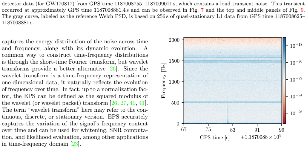
"By examining Figs. 6 and 7, we observe spurious sharp spectral lines in the median wavelet packet PSD near 20 Hz, 500 Hz, and 1600 Hz. We therefore conclude that the sym wavelet family is not suitable for WPT of GW data. The WDM wavelet basis ... is better suited for this PSD estimation task [23, 24]. ... For comparison, the green curve in Fig. 8 shows the result obtained using the median periodogram method. ... the median WDM PSD is more robust [24]."
The WDM wavelet is adopted only after the same GW170817 L1 stretch used in Fig. 8 is found to produce artifacts with sym20. The robustness comparison between median WDM PSD and median periodogram PSD is then performed on this same stretch, so the conclusion is selected post hoc on the evaluation data rather than predicted out of sample. This is a data-dependent model choice, not an equation-level reduction, but it makes the reported robustness an in-sample result.
full rationale
The stationary-noise derivation is not circular in its core mathematics: Eq. (9) is a standard asymptotic result for the log-periodogram, and wavelet thresholding with GGD-modeled detail coefficients is a standard technique. The circularity is confined to the validation loop: the significance level s is calibrated on the same 32 s GW150914 H1 segment so that Var[ϵ] matches π2/6, and the same s and data are then used to demonstrate the Gumbel agreement and to report performance. This makes the distributional check partly self-fulfilling, though the matched-filter SNR and Q improvements are not directly optimized by the s choice. For non-stationary noise, choosing WDM after observing sym20 artifacts on the same GW170817 stretch and then comparing WDM with the median periodogram on that same stretch is a post hoc, in-sample evaluation rather than a forced circularity. The paper is otherwise self-contained, uses public LIGO data, and relies on external references for the wavelet machinery, so the overall circularity is moderate.
Assumptions & free parameters
free parameters (7)
- significance level s =
0.12 (stationary); varied 0.10-0.50 in Table III
- Tukey window alpha =
0.08
- DWT decomposition level m =
6
- wavelet basis (stationary) =
sym7
- wavelet basis (non-stationary) =
sym20 then WDM
- normalization factor for median wavelet packet PSD =
unspecified
- soft thresholding vs hard =
soft
assumptions (6)
- standard math Asymptotic periodogram distribution: Pxx(f) ~ Sxx(f) * chi^2/2 for interior frequencies (Eq. 8)
- standard math Log-periodogram model: ln Pxx + gamma = ln Sxx + eps, with eps Gumbel, variance pi^2/6 (Eqs. 9-10)
- domain assumption Detail coefficients of log-periodogram follow generalized Gaussian distribution (Eq. 11)
- domain assumption Median of wavelet packet coefficients in each frequency bin gives a valid PSD estimate for non-stationary noise
- standard math Squared modulus of wavelet transform equals evolutionary power spectrum up to normalization
- domain assumption Reconstruction with thresholded coefficients recovers log-PSD without bias
Cite this review
Pith. "Pith review of Wavelets for power spectral density estimation of gravitational wave data." pith.science (2026). https://pith.science/paper/2Y5PRXLU
@misc{pith2026250811938,
  author       = {Pith},
  title        = {Pith review of: Wavelets for power spectral density estimation of gravitational wave data},
  year         = {2026},
  howpublished = {\url{https://pith.science/paper/2Y5PRXLU}},
  note         = {Machine review of arXiv:2508.11938}
}
read the original abstract
Power spectral density (PSD) estimation is a critical step in gravitational wave (GW) detectors data analysis. The Welch method is a typical non-parametric spectral estimation approach that estimates the PSD of stationary noise by averaging periodograms of several time segments, or by taking the median of periodograms to adapt to non-stationary noise. In this work, we propose a wavelet-based approach for fast PSD estimation of both stationary and non-stationary noise. For stationary noise, we apply wavelet smoothing to the periodogram, avoiding the segmentation step in the Welch method, and enabling PSD estimates with high frequency resolution and low variance. The wavelet smoothing PSD outperforms Welch PSD in matched filtering and parameter estimation. For non-stationary noise, we estimate the PSD by taking the median of wavelet packet coefficients in each frequency bin, which offers greater robustness than the traditional median periodogram method. This work introduces a new PSD estimation approach for GW data analysis and expands the application of wavelet methods in this field.
Figures


Figures from the paper (6 more)




Reference graph
Works this paper leans on
-
[1]
J. D. E. Creighton and W. G. Anderson, Gravitational- Wave Physics and Astronomy (John Wiley & Sons, Ltd,
-
[2]
P. Jaranowski and A. Krolak, Analysis of Gravitational- Wave Data, Cambridge Monographs on Particle Physics, Nuclear Physics and Cosmology (Cambridge University Press, 2009)
work page 2009
-
[3]
B. P. Abbott et al. (LIGO Scientific and Virgo Collab- oration), A guide to LIGO-Virgo detector noise and ex- traction of transient gravitational-wave signals, Classical and Quantum Gravity 37, 055002 (2020)
work page 2020
-
[4]
B. P. Abbott et al.(LIGO Scientific and Virgo Collabora- tion), GW150914: First results from the search for binary black hole coalescence with Advanced LIGO, Phys. Rev. D 93, 122003 (2016)
work page 2016
- [5]
- [6]
-
[7]
P. Stoica and R. L. Moses, Spectral analysis of signals (Prentice Hall, 2005)
work page 2005
-
[8]
J. G. Proakis and D. G. Manolakis, Digital Signal Pro- cessing: Principles, Algorithms and Applications(Pren- tice Hall, 2007)
work page 2007
Show all 45 references
-
[9]
P. Welch, The use of fast Fourier transform for the esti- mation of power spectra: A method based on time aver- aging over short, modified periodograms, IEEE Transac- tions on Audio and Electroacoustics 15, 70 (1967)
1967
-
[10]
Aasi et al
J. Aasi et al. (LIGO Scientific and Virgo Collaboration), Parameter estimation for compact binary coalescence sig- nals with the first generation gravitational-wave detector network, Phys. Rev. D 88, 062001 (2013)
2013
-
[11]
Veitch et al., Parameter estimation for compact bina- ries with ground-based gravitational-wave observations using the LALInference software library, Phys
J. Veitch et al., Parameter estimation for compact bina- ries with ground-based gravitational-wave observations using the LALInference software library, Phys. Rev. D 91, 042003 (2015)
2015
-
[12]
Wang, J.-B
C.-W.-Z. Wang, J.-B. Zhu, G.-Q. Huang, and F.-W. Shu, Testing the first law of black hole mechanics with gravita- tional waves, Sci. China Phys. Mech. Astron. 67, 100413 (2024)
2024
-
[13]
Ashton et al., Bilby: A User-friendly Bayesian In- ference Library for Gravitational-wave Astronomy, The Astrophysical Journal Supplement Series 241, 27 (2019)
G. Ashton et al., Bilby: A User-friendly Bayesian In- ference Library for Gravitational-wave Astronomy, The Astrophysical Journal Supplement Series 241, 27 (2019)
2019
-
[14]
C. M. Biwer, C. D. Capano, S. De, M. Cabero, D. A. Brown, A. H. Nitz, and V. Raymond, PyCBC Inference: A Python-based Parameter Estimation Toolkit for Com- pact Binary Coalescence Signals, Publications of the As- tronomical Society of the Pacific 131, 024503 (2019)
2019
-
[15]
Cuoco, G
E. Cuoco, G. Cella, and G. M. Guidi, Whitening of non- stationary noise from gravitational wave detectors, Clas- sical and Quantum Gravity 21, S801 (2004)
2004
-
[16]
Cuoco, G
E. Cuoco, G. Calamai, L. Fabbroni, G. Losurdo, M. Maz- zoni, R. Stanga, and F. Vetrano, On-line power spectra identification and whitening for the noise in interferomet- ric gravitational wave detectors, Classical and Quantum Gravity 18, 1727 (2001)
2001
-
[17]
S. Kim, C. Y. Hui, J. Yan, A. P. Leung, K. Oh, A. K. H. Kong, L. C.-C. Lin, and K.-L. Li, Autoregressive search of gravitational waves: Denoising, Phys. Rev. D 109, 102003 (2024)
2024
-
[18]
T. B. Littenberg and N. J. Cornish, Bayesian inference for spectral estimation of gravitational wave detector noise, Phys. Rev. D 91, 084034 (2015)
2015
-
[19]
Gupta and N
T. Gupta and N. J. Cornish, Bayesian power spectral estimation of gravitational wave detector noise revisited, Phys. Rev. D 109, 064040 (2024)
2024
-
[20]
N. J. Cornish and T. B. Littenberg, Bayeswave: Bayesian inference for gravitational wave bursts and instrument glitches, Classical and Quantum Gravity 32, 135012 (2015)
2015
-
[21]
Chatziioannou, C.-J
K. Chatziioannou, C.-J. Haster, T. B. Littenberg, W. M. Farr, S. Ghonge, M. Millhouse, J. A. Clark, and N. Cor- 11 nish, Noise spectral estimation methods and their impact on gravitational wave measurement of compact binary mergers, Phys. Rev. D 100, 104004 (2019)
2019
-
[22]
Christensen and R
N. Christensen and R. Meyer, Parameter estimation with gravitational waves, Rev. Mod. Phys. 94, 025001 (2022)
2022
-
[23]
N. J. Cornish, Time-frequency analysis of gravitational wave data, Phys. Rev. D 102, 124038 (2020)
2020
-
[24]
Necula, S
V. Necula, S. Klimenko, and G. Mitselmakher, Transient analysis with fast Wilson-Daubechies time-frequency transform, Journal of Physics: Conference Series 363, 012032 (2012)
2012
-
[25]
Daubechies, Ten Lectures on Wavelets(Society for In- dustrial and Applied Mathematics, Philadelphia, 1992)
I. Daubechies, Ten Lectures on Wavelets(Society for In- dustrial and Applied Mathematics, Philadelphia, 1992)
1992
-
[26]
Mallat, A Wavelet Tour of Signal Processing: The Sparse Way, 3rd ed
S. Mallat, A Wavelet Tour of Signal Processing: The Sparse Way, 3rd ed. (Academic Press, Inc., USA, 2008)
2008
-
[27]
Torrence and G
C. Torrence and G. P. Compo, A Practical Guide to Wavelet Analysis, Bulletin of the American Meteorolog- ical Society 79, 61 (1998)
1998
-
[28]
Roy, Nonorthogonal wavelet transformation for recon- structing gravitational wave signals, Phys
S. Roy, Nonorthogonal wavelet transformation for recon- structing gravitational wave signals, Phys. Rev. Res. 4, 033078 (2022)
2022
-
[29]
G. P. Nason and B. W. Silverman, The Stationary Wavelet Transform and some Statistical Applications, in Wavelets and Statistics(Springer New York, New York, NY, 1995) pp. 281–299
1995
-
[30]
Cardinali and G
A. Cardinali and G. P. Nason, Locally Stationary Wavelet Packet Processes: Basis Selection and Model Fitting, Journal of Time Series Analysis 38, 151 (2017)
2017
-
[31]
D. B. Percival and A. T. Walden, Wavelet Methods for Time Series Analysis, Cambridge Series in Statistical and Probabilistic Mathematics (Cambridge University Press, 2000)
2000
-
[32]
Moulin, Wavelet thresholding techniques for power spectrum estimation, IEEE Transactions on Signal Pro- cessing 42, 3126 (1994)
P. Moulin, Wavelet thresholding techniques for power spectrum estimation, IEEE Transactions on Signal Pro- cessing 42, 3126 (1994)
1994
-
[33]
Sysel and Z
P. Sysel and Z. Sm´ ekal, Enhanced estimation of power spectral density of noise using the wavelet transform, in Personal Wireless Communications(Springer US, 2007) pp. 521–532
2007
-
[34]
Vidakovic, Statistical Modeling by Wavelets(John Wi- ley & Sons, Inc., 1999)
B. Vidakovic, Statistical Modeling by Wavelets(John Wi- ley & Sons, Inc., 1999)
1999
-
[35]
D. R. Brillinger, Time Series: Data Analysis and Theory (Society for Industrial and Applied Mathematics, 2001)
2001
-
[36]
M. S. Bartlett and D. G. Kendall, The Statistical Analy- sis of Variance-Heterogeneity and the Logarithmic Trans- formation, Supplement to the Journal of the Royal Sta- tistical Society 8, 128 (1946)
1946
-
[37]
S. G. Mallat, A theory for multiresolution signal decom- position: the wavelet representation, IEEE Transactions on Pattern Analysis and Machine Intelligence 11, 674 (1989)
1989
-
[38]
D. L. Donoho and I. M. Johnstone, Ideal Spatial Adap- tation by Wavelet Shrinkage, Biometrika 81, 425 (1994)
1994
-
[39]
M. B. Priestley, Evolutionary Spectra and Non- Stationary Processes, Journal of the Royal Statistical So- ciety: Series B (Methodological) 27, 204 (2018)
2018
-
[40]
G. P. Nason, R. von Sachs, and G. Kroisandt, Wavelet Processes and Adaptive Estimation of the Evolutionary Wavelet Spectrum, Journal of the Royal Statistical Soci- ety. Series B (Statistical Methodology) 62, 271 (2000)
2000
-
[41]
S. V. Bellegem and R. von Sachs, Locally adaptive es- timation of evolutionary wavelet spectra, The Annals of Statistics 36, 1879 (2008)
2008
-
[42]
G. R. Lee, R. Gommers, F. Wasilewski, K. Wohlfahrt, and A. O’Leary, PyWavelets: A Python package for wavelet analysis, Journal of Open Source Software 4, 1237 (2019)
2019
-
[43]
Cornish, Wdm transform (2020)
N. Cornish, Wdm transform (2020)
2020
-
[44]
Digman, Wdmwavelettransforms (2023)
M. Digman, Wdmwavelettransforms (2023)
2023
-
[2011]
Chap. 7, pp. 269–347
Reviewed August 5, 2026 · model on record in the stance chip above.
Discussion (0). Continue with ORCID to comment.