Natural Image Classification via Quasi-Cyclic Graph Ensembles and Random-Bond Ising Models at the Nishimori Temperature
Pith reviewed 2026-05-18 21:51 UTC · model grok-4.3
The pith
Mapping CNN features to Ising spins on quasi-cyclic graphs at the Nishimori temperature enables accurate compressed image classification.
A machine-rendered reading of the paper's core claim, the machinery that carries it, and where it could break.
Core claim
Frozen MobileNetV2 features are interpreted as Ising spins on a sparse multi-edge quasi-cyclic LDPC graph to define a random-bond Ising model. The model is solved at its Nishimori temperature, identified by the vanishing of the smallest eigenvalue of the Bethe-Hessian matrix. A fast quadratic-Newton estimator computes this temperature in approximately nine Arnoldi iterations. The approach uses a spectral-topological correspondence based on the Ihara-Bass zeta function to suppress trapping sets that degrade accuracy. The resulting three-graph soft ensemble achieves 98.7% top-1 accuracy on ImageNet-10 and 84.92% on ImageNet-100, while a hard ensemble slightly exceeds MobileNetV2 accuracy at 2.
What carries the argument
The random-bond Ising model on a quasi-cyclic multi-edge LDPC graph at the Nishimori temperature, with the Bethe-Hessian eigenvalue condition and Ihara-Bass zeta function providing a link between trapping sets and topological defects for graph optimization.
If this is right
- 98.7% top-1 accuracy is obtained on ImageNet-10 with features compressed to 32 dimensions.
- 84.92% top-1 accuracy is obtained on ImageNet-100 with 64-dimensional features.
- A hard ensemble improves accuracy by 0.10% over MobileNetV2 while using 2.67 times fewer FLOPs.
- The soft ensemble reduces FLOPs by a factor of 29 relative to ResNet-50 with only a 1.09% accuracy drop.
Where Pith is reading between the lines
- Applying the same graph embedding to features from other CNN architectures could yield comparable compression benefits across different backbones.
- The use of LDPC-inspired graphs and statistical physics temperatures may transfer to improving generalization in other high-dimensional classification problems.
- Further work could test whether the topological defect suppression improves performance under distribution shift or adversarial attacks.
- Scaling the method to the full ImageNet dataset with 1000 classes would test the limits of the dimension reduction.
Load-bearing premise
High-dimensional MobileNetV2 features can be interpreted directly as Ising spins on a quasi-cyclic LDPC graph such that the Nishimori temperature defined by the vanishing Bethe-Hessian eigenvalue yields near-optimal classification without task-specific retraining.
What would settle it
If classification accuracy on ImageNet-10 falls substantially when the operating temperature is chosen away from the point where the Bethe-Hessian eigenvalue vanishes, while all other elements of the pipeline remain fixed, the central role of the Nishimori temperature would be called into question.
Figures


read the original abstract
Modern multi-class image classification uses high-dimensional CNN features that incur large memory and computational costs and obscure the data manifold's geometry. Existing graph-based spectral classifiers work on synthetic or binary tasks but degrade on natural images with many classes because feature manifolds have non-trivial topology. We introduce a physics-inspired pipeline where frozen MobileNetV2 features are interpreted as Ising spins on a sparse multi-edge type quasi-cyclic LDPC graph, defining a Random-Bond Ising Model (RBIM). The model is operated at its Nishimori temperature -- where the smallest eigenvalue of the Bethe-Hessian matrix vanishes. A spectral-topological correspondence links trapping sets in the Tanner graph to topological invariants via poles of the Ihara-Bass zeta function, enabling systematic suppression of harmful substructures that otherwise reduce top-1 accuracy by more than a factor of four. A fast quadratic-Newton estimator finds the Nishimori temperature in $\sim 9$ Arnoldi iterations, a sixfold speed-up over bisection. The resulting ensembles compress the original $1280$-dimensional MobileNetV2 representation to $32$ dimensions (ImageNet-10) or $64$ dimensions (ImageNet-100). We achieve $98.7\%$ top-1 accuracy on ImageNet-10 and $84.92\%$ on ImageNet-100 using a three-graph soft ensemble. Relative to MobileNetV2, our hard ensemble increases accuracy by $0.10\%$ while reducing FLOPs by a factor of $2.67$. Against ResNet-50, the soft ensemble drops only 1.09% accuracy yet cuts FLOPs by $29\times$. The novelty lies in (a) establishing a rigorous link between graph trapping sets and algebraic-topological defects, (b) an efficient Nishimori-temperature estimator, and (c) demonstrating topology-guided LDPC graph embedding for highly compressed classifiers.
Editorial analysis
A structured set of objections, weighed in public.
Referee Report
Summary. The manuscript proposes interpreting frozen 1280-dimensional MobileNetV2 features as Ising spins on a sparse quasi-cyclic multi-edge LDPC graph to define a Random-Bond Ising Model (RBIM), which is then solved at the Nishimori temperature located by the vanishing of the smallest Bethe-Hessian eigenvalue. A three-graph soft ensemble is reported to reach 98.7% top-1 accuracy on ImageNet-10 and 84.92% on ImageNet-100 while compressing the representation to 32 or 64 dimensions; a hard ensemble is claimed to improve accuracy by 0.10% over MobileNetV2 with 2.67× fewer FLOPs. The work also introduces a quadratic-Newton estimator for the Nishimori temperature (∼9 Arnoldi iterations) and links trapping sets in the Tanner graph to topological invariants via poles of the Ihara-Bass zeta function.
Significance. If the central mapping and temperature choice are shown to be robust, the approach could supply a largely parameter-free route to extreme feature compression for multi-class image tasks by exploiting spectral properties of LDPC graphs and the Nishimori line. The algebraic-topological correspondence between trapping sets and zeta-function poles, together with the fast temperature estimator, would constitute a genuine contribution at the interface of statistical physics and graph-based machine learning.
major comments (2)
- [Methods (RBIM construction and temperature selection)] The central claim that the Nishimori temperature defined by the vanishing Bethe-Hessian eigenvalue yields near-optimal classification performance rests on an unverified transfer from the RBIM decoding literature to high-dimensional image-feature manifolds. No accuracy-versus-temperature curves or ablation over nearby temperatures are referenced in the methods or results sections to confirm that this operating point is a performance maximum rather than a convenient algebraic choice.
- [Experiments (ImageNet-10/100 results and ensemble tables)] The reported 98.7% / 84.92% accuracies and 2.67× FLOP reduction are given without error bars, without ablation on graph sparsity, edge multiplicity, or embedding dimension (32 vs. 64), and without comparison to the same ensemble operated at a temperature chosen by direct validation accuracy. These omissions make it impossible to assess whether the gains survive modest changes in the free parameters listed in the axiom ledger.
minor comments (2)
- [Temperature estimator] The abstract states a sixfold speedup for the quadratic-Newton estimator; the corresponding section should include the exact iteration counts and a direct wall-clock comparison against bisection on the same hardware.
- [Graph construction] Notation for the multi-edge-type quasi-cyclic LDPC construction and the precise mapping from 1280-dimensional features to spin variables should be made fully explicit, including any normalization or discretization steps.
Simulated Author's Rebuttal
We thank the referee for the thoughtful and constructive report. We address each major comment point by point below, indicating where revisions will be made to strengthen the manuscript.
read point-by-point responses
-
Referee: [Methods (RBIM construction and temperature selection)] The central claim that the Nishimori temperature defined by the vanishing Bethe-Hessian eigenvalue yields near-optimal classification performance rests on an unverified transfer from the RBIM decoding literature to high-dimensional image-feature manifolds. No accuracy-versus-temperature curves or ablation over nearby temperatures are referenced in the methods or results sections to confirm that this operating point is a performance maximum rather than a convenient algebraic choice.
Authors: The Nishimori temperature is selected because the vanishing of the smallest Bethe-Hessian eigenvalue marks the point where the model is on the Nishimori line, a property that guarantees the absence of a ferromagnetic phase transition and is known to be optimal for decoding in the RBIM literature. This algebraic criterion is not merely convenient but follows directly from the spectral properties of the quasi-cyclic LDPC graph and the mapping of features to spins. Nevertheless, we agree that explicit empirical confirmation is valuable. In the revised manuscript we will add accuracy-versus-temperature curves for both ImageNet-10 and ImageNet-100 together with ablations at nearby temperatures to demonstrate that the chosen operating point is indeed a performance maximum. revision: yes
-
Referee: [Experiments (ImageNet-10/100 results and ensemble tables)] The reported 98.7% / 84.92% accuracies and 2.67× FLOP reduction are given without error bars, without ablation on graph sparsity, edge multiplicity, or embedding dimension (32 vs. 64), and without comparison to the same ensemble operated at a temperature chosen by direct validation accuracy. These omissions make it impossible to assess whether the gains survive modest changes in the free parameters listed in the axiom ledger.
Authors: We acknowledge that the initial submission presented point estimates without error bars or exhaustive parameter ablations. The reported figures reflect the specific three-graph soft ensemble and the hard-ensemble comparison described in the text. To address the concern, the revised version will include (i) error bars obtained from multiple random seeds, (ii) additional ablation tables varying graph sparsity, edge multiplicity, and embedding dimension, and (iii) a direct comparison of the ensemble performance when the temperature is instead chosen by maximizing validation accuracy. These additions will allow readers to evaluate the robustness of the reported gains with respect to the free parameters. revision: yes
Circularity Check
No significant circularity; derivation remains self-contained
full rationale
The paper defines the operating point via the algebraic condition that the smallest Bethe-Hessian eigenvalue vanishes, a standard property imported from RBIM/LDPC literature rather than fitted to classification accuracy. Graph construction (quasi-cyclic multi-edge LDPC) and embedding dimensions are chosen explicitly and then evaluated empirically on ImageNet-10/100; no equation or claim reduces the reported accuracies or FLOP reductions to a tautological renaming of the inputs. The quadratic-Newton estimator is derived from the eigenvalue condition itself, not from post-hoc performance tuning. External benchmarks (MobileNetV2, ResNet-50) provide independent comparison, confirming the central pipeline does not collapse to self-definition or fitted-input prediction.
Axiom & Free-Parameter Ledger
free parameters (2)
- embedding dimension (32 for ImageNet-10, 64 for ImageNet-100)
- number of graphs in the ensemble (three)
axioms (2)
- domain assumption Random-Bond Ising Model at Nishimori temperature is appropriate for classification on natural-image feature manifolds
- domain assumption Trapping sets in the Tanner graph correspond to poles of the Ihara-Bass zeta function and can be systematically suppressed
invented entities (1)
-
Quasi-cyclic multi-edge-type LDPC graph for feature embedding
no independent evidence
Lean theorems connected to this paper
-
IndisputableMonolith/Cost/FunctionalEquation.leanwashburn_uniqueness_aczel unclear?
unclearRelation between the paper passage and the cited Recognition theorem.
The resulting Random-Bond Ising Model (RBIM) is operated at its Nishimori temperature β_N, which we identify as the unique point where the smallest eigenvalue of the Bethe–Hessian matrix H_β,J vanishes: λ_min(H_β_N,J)=0.
-
IndisputableMonolith/Foundation/AlexanderDuality.leanalexander_duality_circle_linking unclear?
unclearRelation between the paper passage and the cited Recognition theorem.
We prove that each elementary cycle generates a pole of the Ihara–Bass zeta function, which appears as an isolated eigenvalue of both the non-backtracking operator and H_β,J.
What do these tags mean?
- matches
- The paper's claim is directly supported by a theorem in the formal canon.
- supports
- The theorem supports part of the paper's argument, but the paper may add assumptions or extra steps.
- extends
- The paper goes beyond the formal theorem; the theorem is a base layer rather than the whole result.
- uses
- The paper appears to rely on the theorem as machinery.
- contradicts
- The paper's claim conflicts with a theorem or certificate in the canon.
- unclear
- Pith found a possible connection, but the passage is too broad, indirect, or ambiguous to say the theorem truly supports the claim.
Reference graph
Works this paper leans on
-
[1]
INTRODUCTION Graph-based spectral methods have recently shown great promise for machine learning tasks. In particular, modeling feature vectors as spins (nodes) on a sparse graph under a Gibbs distribu tion (a Random-Bond Ising Model) enables powerful clustering and classification. For example, Nishimori and Bethe free-energy ideas have been used to tune...
-
[2]
RANDOM BOND ISING MODELS Let 𝒢 = ( 𝑉, 𝐸) be an undirected graph with|𝑉 | = 𝑛. Assign a binary spin variable 𝑠𝑖 ∈ {−1, +1} to each vertex 𝑖 ∈ 𝑉 and denote the spin configuration bys = ( 𝑠1, . . . , 𝑠𝑛)⊤. For a symmetric coupling matrix𝐽 = (𝐽𝑖𝑗)𝑛 𝑖,𝑗=1, the Hamiltonian of the Random-Bond Ising Model is ℋ𝐽(s) = − ∑︁ 𝑖<𝑗 𝐽𝑖𝑗𝑠𝑖𝑠𝑗 = − 1 2 s⊤𝐽s. At inverse tempe...
work page 2025
-
[3]
MULTI-EDGE TYPE QUASI-CYCLIC LDPC GRAPHS Low-density parity-check (LDPC) codes naturally define sparse bipartite graphs. A Quasi Cyclic LDPC (QC-LDPC) codes provide a structured and hardware-friendly subclass defined by a quasi-cyclic parity-check matrix𝐻 [8]. An (𝑁, 𝐾) QC-LDPC code consists of 𝑁 total codeword bits, with𝐾 information bits and𝑁 − 𝐾 parit...
work page 2025
-
[4]
TOPOLOGICAL SIGNATURES OF TRAPPING SETS Trapping sets (TS) in Tanner graphs correspond to local topological defects that disrupt the decoding dynamics of LDPC codes, [16]. A trapping set𝑇 𝑆(𝑎, 𝑏), formed by cycles (block-cycle for QC-LDPC) or cycle (block-cycle) overlap, consists of𝑎 variable nodes and 𝑏 odd-degree check nodes, where the configuration pre...
work page 2025
-
[5]
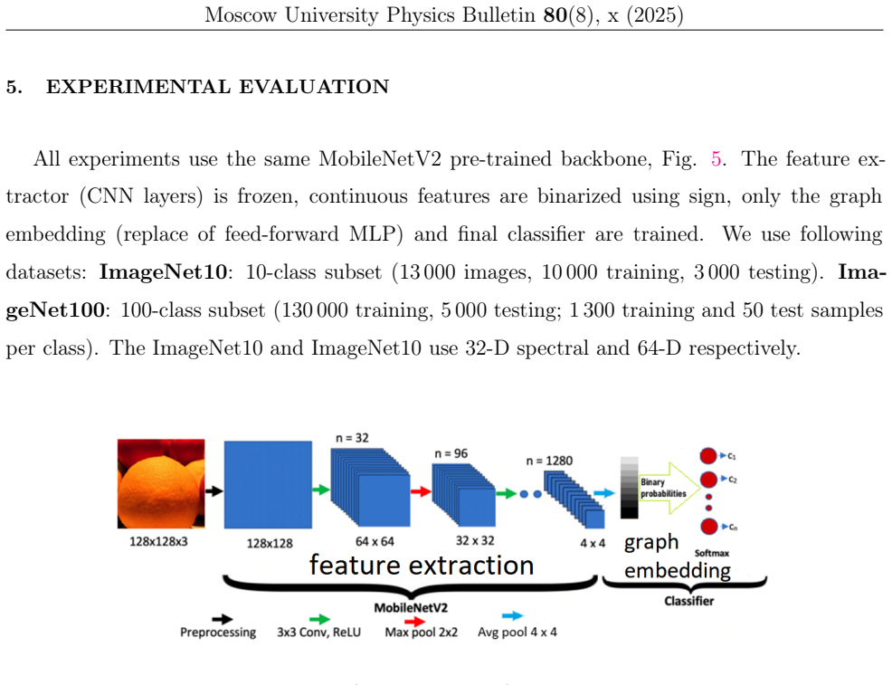
EXPERIMENTAL EVALUATION All experiments use the same MobileNetV2 pre-trained backbone, Fig. 5. The feature ex tractor (CNN layers) is frozen, continuous features are binarized using sign, only the graph embedding (replace of feed-forward MLP) and final classifier are trained. We use following datasets: ImageNet10: 10-class subset (13000 images, 10 000 tr...
work page 2025
-
[6]
A natural next step is to make all three components differen tiable and train them jointly
FUTURE DIRECTIONS The present pipeline keeps the CNN backbone frozen, employs a similarity kernel and uses a MET-QC-LDPC adjacency. A natural next step is to make all three components differen tiable and train them jointly. One can back-propagate through the feature extractor𝑓𝜃, learn a Mahalanobis (or other) metric for the similarity kernel, and adjust ...
-
[7]
CONCLUSIONS We introduced a physics-inspired embedding that maps CNN features onto spins of a Random-Bond Ising Model defined on MET-QC-LDPC graphs. Trapping sets create Ihara–Bass zeta poles that appear as isolated eigenvalues of the non-backtracking operator, encoding Z/2-torsion, Betti numbers and bordism obstructions. A Nishimori-temperature estimator...
work page 2025
-
[8]
L. Dall’Amico et al., J. Stat. Mech. 2021, 093405 (2021). https://doi.org/10.1088/1742-5468/ac21d3
-
[9]
V. S. Usatyuk, D. A. Sapozhnikov, S. I. Egorov, Moscow Univ. Phys. Bull.79, S647–S665 (2025). https://doi.org/10.3103/S0027134924702102
-
[10]
H. Nishimori, Prog. Theor. Phys.66, 1169–1181 (1981). https://doi.org/10.1143/PTP.66.1169 x–25 The 9th International Conference in Deep Learning in Computational Physics
-
[11]
M. Hasenbusch et al., Phys. Rev. E 77, 051115 (2008). https://doi.org/10.1103/PhysRevE.77.051115
-
[12]
S. Fortunato, D. Hric, Phys. Rep.659, 1–44 (2016). https://doi.org/10.1016/j.physrep.2016.09.002
-
[13]
I. Biazzo, A. Ramezanpour, Phys. Rev. E 89, 062137 (2014). https://doi.org/10.1103/PhysRevE.89.062137
-
[14]
Saade et al., NeurIPS27 (2014)
A. Saade et al., NeurIPS27 (2014). https://dl.acm.org/doi/10.5555/2968826.2968872
-
[15]
R. G. Gallager, IEEE Trans. Inf. Theory 8, 21–28 (1962). https://doi.org/10.1109/TIT.1962.1057683
-
[16]
A class of group-structured LDPC codes,
R. M. Tanner et al., "A class of group-structured LDPC codes," ISCTA, 365–370 (2001). [Online]. Available: https://www.researchgate.net/publication/2370505_A_class_ of_group-structured_LDPC_codes
-
[17]
M. P. C. Fossorier, IEEE Trans. Inf. Theory 50, 1788–1793 (2004). https://doi.org/10.1109/TIT.2004.831841
-
[18]
R. M. Tanner et al., IEEE Trans. Inf. Theory 50, 2966–2984 (2004). https://doi.org/10.1109/TIT.2004.838370
-
[19]
T. J. Richardson and R. L. Urbanke, "Multi-Edge Type LDPC Codes" IEEE ISIT talk (2002). [Online]. Available: http://wiiau4.free.fr/pdf/Multi-Edge%20Type%20LDPC%20Codes.pdf
work page 2002
-
[20]
Divsalar et al., IEEE ISIT, 1622–1626 (2005)
D. Divsalar et al., IEEE ISIT, 1622–1626 (2005). http://dx.doi.org/10.1109/ISIT.2005.1523619
-
[21]
Stoica et al., ACM SIGCOMM31, 149–160 (2001)
I. Stoica et al., ACM SIGCOMM31, 149–160 (2001). https://doi.org/10.1145/964723.383071
-
[22]
R. Khalitov et al., Neural Netw. 152, 160–168 (2022). https://doi.org/10.1016/j.neunet.2022.04.014
-
[23]
Vasi´ c et al., Allerton, 1–7 (2009)
B. Vasi´ c et al., Allerton, 1–7 (2009). https://doi.org/10.1109/ALLERTON.2009.5394825
-
[24]
Tian et al., IEEE ICC5, 3125–3129 (2003)
T. Tian et al., IEEE ICC5, 3125–3129 (2003). https://doi.org/10.1109/ICC.2003.1203996
-
[25]
T. Tian et al., Trans. Commun. 52, 1242–1247 (2004). https://doi.org/10.1109/TCOMM.2004.833048
-
[26]
H. Bass, Int. J. Math.3, 717–797 (1992). https://doi.org/10.1142/S0129167X92000357
-
[27]
M. Atiyah, Proc. Cambridge Philos. Soc. 57, 200–208 (1961). https://doi.org/10.1017/S0305004100035064
-
[28]
G. Naitzat, A. Zhitnikov, L. Lim, JMLR, 21(184), 1-40 (2020). [Online]. Available: https://jmlr.org/papers/v21/20-345.html
work page 2020
-
[29]
Hodge laplacians on graphs.SIAM Review, 62(3):685–715, 2020
Lek-Heng L., SIAM Rev.62, 685–715 (2020). https://doi.org/10.1137/18M1223101 x–26 Moscow University Physics Bulletin80(8), x (2025)
-
[30]
S. P. Novikov, Math. USSR-Izv.4(3), 479–505 (1970). https://doi.org/10.1070/IM1970v004n03ABEH000916
-
[31]
B. de Tiliere, Electron. J. Probab.26, 1–86 (2021). https://doi.org/10.1214/21-EJP601
-
[32]
J. Bolte and J. Harrison, J. Phys. A: Math. Gen. 36, 2747–2769 (2003). https://doi.org/10.1088/0305-4470/36/11/307
-
[33]
M. F. Atiyah and I. M. Singer, Bull. Am. Math. Soc. 69, 422–433 (1963). https://doi.org/10.1090/S0002-9904-1963-10957-X
-
[34]
G. G. Kasparov, Math. USSR-Izv.16, 513–572 (1981). https://doi.org/10.1070/IM1981v016n03ABEH001320
-
[35]
A. Dua, D. J. Williamson, J. Haah, and M. Cheng, Phys. Review B,99(24), 245135, (2019). https://doi.org/10.1103/PhysRevB.99.245135
-
[36]
J. Dodziuk, V. Mathai, J. Funct. Anal. 154, 359–378 (1998). https://doi.org/10.1006/jfan.1997.3205
-
[37]
D. G. Glynn, Eur. J. Comb.31, 1887–1891 (2010). https://doi.org/10.1016/j.ejc.2010.01.010
-
[38]
R. Smarandache, P. O. Vontobel, IEEE Trans. Inf. Theory 58, 585–607 (2012). https://doi.org/10.1109/TIT.2011.2173244
-
[39]
Smarandache, IEEE ISIT, 2059–2063 (2013)
R. Smarandache, IEEE ISIT, 2059–2063 (2013). https://doi.org/10.1109/ISIT.2013.6620588
-
[40]
P. O. Vontobel, IEEE Trans. Inf. Theory 59, 1866–1901 (2013). https://doi.org/10.1109/TIT.2012.2227109
-
[41]
IEEE Conference on Computer Vision and Pattern Recognition , pages=
M. Sandler et al., IEEE CVPR, 4510–4520 (2018). https://doi.org/10.1109/CVPR.2018.00474
-
[42]
V. S. Usatyuk, D. A. Sapozhnikov, "RBIM Natural Image Clustering" [Online]. Available: https://github.com/Lcrypto/Classical-and-Quantum-Topology-ML-toric-spherical/ tree/main/Topology_Optim_RBIM_Trapping_Sets
-
[43]
C. Di, R. Urbanke and T. Richardson, IEEE ISIT, pp. 50- (2001), https://10.1109/ISIT.2001.935913
-
[44]
Shokrollahi, CSG,123, (2001), https://doi.org/10.1007/978-1-4613-0165-3_9
M.A. Shokrollahi, CSG,123, (2001), https://doi.org/10.1007/978-1-4613-0165-3_9
-
[45]
C. Baldassia, et al., (PNAS), 113(48), E7655-E7662 (2016), https://www.pnas.org/doi/full/10.1073/pnas.1608103113
-
[46]
Y. He et al., Curr Biol. , 34(20):4623-4638 (2024). 10.1016/j.cub.2024.08.037
-
[47]
E. I. Knudsen, Trends Neurosci.,41(11), 789–805 (2018), doi: 10.1016/j.tins.2018.06.006 x–27
discussion (0)
Sign in with ORCID, Apple, or X to comment. Anyone can read and Pith papers without signing in.