Objective Value Change and Shape-Based Accelerated Optimization for the Neural Network Approximation

Pengcheng Xie; Zihao Zhou; Zijian Zhou

REVIEW 3 major objections 5 minor 45 references

Objective Value Change and Shape-Based Accelerated Optimization for the Neural Network Approximation

T0 review · 3 major / 5 minor · reviewed 2026-08-15 · deepseek-v4-flash

Challenge this review Re-run · record.json Download PDF Read on arXiv ↗ Review JSON

Pith's one-line read The paper proposes a new local descriptor of an objective function, VC (value change), defined as the maximum difference between two values of the function inside a box of side length $L$ around a point.

desk verdict Plausible VC-error correlation and a useful residual-subtraction trick, but the minority-tendency claim is unsupported and the theory as stated contains a false proposition. read the letter →

arxiv 2508.20290 v1 pith:HJ7DQXJ4 submitted 2025-08-27 cs.LG cs.AIcs.NAmath.NAmath.OC

Pengcheng Xie , Zihao Zhou , Zijian Zhou This is my paper · ORCID

classification cs.LGcs.AIcs.NAmath.NAmath.OC MSC 68T0741A2565D15

keywords valuechangeVCdensityVC-tendencyminority-tendencyIVCdistanceneuralnetworkapproximationpreprocessingkernelestimation

verification ladder T0 review T1 audit T2 compute T3 formal

The pith

A machine-rendered reading of the paper's core claim, the machinery that carries it, and where it could break.

The reading

The paper proposes a new local descriptor of an objective function, VC (value change), defined as the maximum difference between two values of the function inside a box of side length $L$ around a point. It claims this descriptor organises neural-network approximation behavior: regions with larger VC retain higher prediction errors throughout training (the VC-tendency), and the distribution of VC values is learned first where its target density is smallest (the minority-tendency). On top of this, the paper defines an integral VC (IVC) distance that measures how much two functions differ in local variation, and uses it to build preprocessing schemes that initialize a network with the target's variation shape before training. The resulting preprocessing accelerates training and improves accuracy on linear functions, monochrome image approximation, and flow past a cylinder. If the tendencies are robust, VC gives a derivative-free, data-only way to predict where a neural approximation will be unreliable and to fix it in advance.

What carries the argument

The central object is the value change $VC_L(f,x)$, the maximum amplitude of $f$ inside a box of side $L$ around $x$; its $L$-dependent derivative recovers $|f'(x)|$ for $C^1$ functions, which is why the paper reads it as a multi-scale, derivative-free generalization of slope. Around this object sit its distribution (VC density), the ratio of two densities (VCDR), and the integrated version $IVC(f,x)$ averaged over $L$, whose spatial integral defines the IVC distance. These objects do the work of translating difficulty into a measurable geometric quantity: VC-tendency connects pointwise error to VC magnitude, the VC density ratio tracks how the approximation progresses in distribution, and the IVC distance provides the objective that the preprocessing algorithm tries to minimize before ordinary training begins.

What would settle it

Rerun the experiments in Tables 4.1 and 4.2 replacing kernel density estimates with histograms of the same VC samples; if the order in which VC levels converge changes, the minority-tendency is an estimator artifact rather than a property of neural network approximation.

Watch

Extended reading notes

Core claim

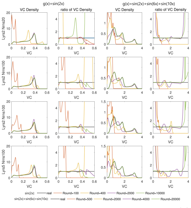
The central claim is that the local variation of the objective function $f$, measured by $VC_L(f,x) = \sup_{y_1,y_2} |f(y_1)-f(y_2)|$ over a box of side $L$ centered at $x$, controls how difficult that neighborhood is to approximate. Experiments on a monochrome image and on flow past a cylinder show that, once pixels are sorted by VC, average, maximum, and median prediction errors increase with VC, and this ordering strengthens as training proceeds. In distributional terms, the paper claims a minority-tendency: comparing the VC density of the network with that of the target, the levels of VC that are rare in the target are the ones whose densities converge first, regardless of whether rare means small VC or large VC. From VC it builds a norm, the IVC distance $Dist_{IVC}(f_1,f_2)=\int_\Omega IVC(f_1-f_2,x)\,dx$, which vanishes exactly when the two functions differ by a constant, and shows that preprocessing that reduces this distance speeds up the later training, with numerical support on linear, image, and cylinder-flow tasks.

Load-bearing premise

The minority-tendency rests on trusting the estimated ratio of two VC density curves even where the target curve is nearly zero; the paper states that the ratio has no reference significance in that regime, and the supporting tables contain many zero and near-zero entries.

Editorial extensions

If this is right

Training behavior of a fixed network can be predicted, up to ordering, from a single static computation of VC over the sampling domain, without simulating training.
High-VC regions, such as edges, discontinuities, and steep gradients, should be expected to hold the largest residual errors, so sampling or capacity should be concentrated there.
Initializing or splitting a training problem so that the network's VC shape matches the target, meaning a small IVC distance, yields faster convergence at equal accuracy, as demonstrated on the three test problems.
The minority-tendency gives a distribution-level description of approximation order that is distinct from low-frequency-first: rare VC levels can converge before common ones.
IVC distance is a genuine metric on functions modulo additive constants, so it can be used as a shape-only similarity measure between a model and a target.

Reading between the lines

Editorial extensions of the paper, not claims the author makes directly.

VC could be used as a sampling or weighting rule: train with points weighted by VC density or by VC magnitude to test whether the observed ordering is a cause or merely a correlation.
The minority-tendency, if real, suggests a curriculum: fit rare VC levels first and common levels later, paralleling but not identical to frequency-based curriculum learning; a direct experiment would be to train on a function whose VC density is deliberately made bimodal and inspect the convergence order of the two modes.
The VCDR tables' zero and $10^{-7}$ entries indicate that the ratio estimator needs regularization, such as additive smoothing or log-density comparison, before the minority-tendency can be tested rigorously; this extends the paper's own caveat into a concrete recommendation.
The IVC distance could double as an online diagnostic: monitoring $Dist_{IVC}(\psi_{NN}, f)$ during training would reveal when the network has stopped improving in shape even while the $L^2$ loss is still decreasing.

Share X Bluesky LinkedIn Reddit HN

Signed reviews

No signed human review yet.

Editorial analysis

A structured set of objections, weighed in public.

Desk editor's note, referee report, and a circularity audit.

Desk Editor's Note

read the letter

Read it carefully. My judgment is close to the reader's, with one adjustment: the paper has a genuinely useful empirical correlation and a sensible preprocessing trick, so it is not a zero. The VC-tendency (larger local variation → larger approximation error) is convincingly shown in Figures 4.2–4.5 for the image and cylinder data. That is consistent with the frequency-principle literature, which the paper cites but never actually connects; that missed connection hurts the novelty claim more than the result. Also, VC_L is just the classical local oscillation of f (sup of |f(y1)-f(y2)| over a box), so presenting it as a new metric is not accurate. The interpolation-subtraction preprocessing (VCP-obj) is reasonable and the experiments suggest it helps.

What is not established is the minority-tendency. The quantitative evidence is Tables 4.1 and 4.2, VCDR values in the regime the paper itself flags as meaningless (Definition 3.9: when true density approaches 0, the ratio has no reference significance). The tables are full of exact 0 and 1e-7 entries, no seeds or KDE bandwidths are reported, and the two examples order convergence in opposite directions by absolute VC; they are reconciled only by relabeling the low-density side as 'minority' after the fact. That claim needs to be redone with density floors, variance across seeds, and a pre-registered notion of minority.

Two technical fixes are needed. Proposition 3.2 is false as stated: for f(x)=-x, VC_L = L for every box, so the L-derivative is 1 while f'=-1. The proof drops the absolute value; the correct statement is |f'|. And Section 2.1's text says f2 (slope 10) has consistently smaller test loss than f1 (slope 1) at 10,000 steps, then concludes smaller slopes converge faster. As written that is backwards; likely a typo, but it should be fixed.

The preprocessing validation is partly circular: Algorithm 5.1 builds the initial model by minimizing DistIVC and then reports that smaller DistIVC correlates with faster convergence. The C-vs-D experiment compares f-g to f-g/2, which is essentially a smaller residual target versus a larger one; ordinary warm-starting could explain the speedup. The IVC distance is a fine heuristic, but it needs a baseline that separates the VC mechanism from residual-size reduction.

For people working on spectral-bias diagnostics or PINN warm-starting, there is useful material here. Bottom line: the VC-tendency correlation and the residual-subtraction preprocessing are worth a serious referee. I would not desk reject. Send to review with the expectation of major revision: fix the proposition, fix Section 2.1, redo minority-tendency properly. If that doesn't happen, reject.

Referee Report

3 major / 5 minor

Summary. The paper proposes a local 'value change' (VC) metric VCL(f,x), a VC density, and an integral VC (IVC) distance, and uses these to characterize neural-network approximation. It claims a VC-tendency (regions with larger VC have larger approximation errors), a minority-tendency (neural networks first match VC density at VC levels that are less frequent in the target function), and a preprocessing framework that minimizes the IVC distance to the objective and thereby accelerates training. The supporting experiments cover linear functions, a monochrome image, flow past a cylinder, and several preprocessing variants.

Significance. If the empirical claims were robust, the VC metric could serve as a useful local diagnostic and preprocessing criterion for neural-network approximation, and the paper does ship code links and performs experiments on nontrivial image and PDE-related data. However, the central theoretical proposition is false as stated, and the quantitative evidence for the minority-tendency is taken from a regime the paper itself declares meaningless. The preprocessing experiments are suggestive but not yet isolated from generic initialization effects. The current manuscript therefore does not establish the claims it emphasizes.

major comments (3)

[Section 3.1, Proposition 3.2] Proposition 3.2 is false as written. For f(x) = -x on [-1,1], one has VCL(f,x0) = L for every x0 and every L, so the right L-derivative of VCL at L = 0 is 1, while f'(x0) = -1. The proof drops absolute values and uses inequalities that do not pass to valid limit bounds in the stated direction. Since Section 3.2 and Section 4 use VC as a tractable proxy for local slope magnitude, this proposition is load-bearing. It should be corrected, at minimum, to the statement that the L-derivative equals |f'(x0)| for differentiable f, and the proof must be rewritten accordingly.
[Section 4.2, Tables 4.1 and 4.2] The minority-tendency evidence is drawn from exactly the regime that Definition 3.9's remark declares to have 'no reference significance': when the true VC density approaches zero, small fluctuations of the neural network's VC density make the VCDR ratio unreliable. Tables 4.1 and 4.2 contain multiple exact 0 entries and values such as 5.7e-8 at early rounds, and no KDE bandwidth, density floor, sample count, or seed variance is reported. A ratio whose numerator or denominator is zero or near zero from a KDE estimate is dominated by bandwidth and finite-sample noise, not by approximation progress. Moreover, the two examples order convergence by absolute VC in opposite directions and are reconciled only by post hoc relabeling of which VC values are the minority. As presented, the claimed minority-tendency ordering is not distinguishable from KDE artifacts and therefore is not established.
[Section 6.1, preprocessing experiments] The comparison of methods A and B does not isolate the effect of DistIVC. Method A starts from a pretrained network that differs from the direct-initialization baseline in both its parameter values and its initial function values, so the faster convergence could be due to favorable initialization or transfer effects more generally. The C-versus-D comparison is better controlled, but the paper's main preprocessing claim would still benefit from a baseline in which the initial model is produced by an alternative criterion unrelated to IVC. Without such a control, the assertion that minimizing IVC distance specifically, rather than any reasonable preprocessing/initialization, drives the acceleration is underdetermined.

minor comments (5)

[Section 2.1] The sentence 'the test loss for the f2 approximation is always smaller than the f1 approximation' contradicts the immediately preceding conclusion that the smaller-slope function f1 converges faster; this is likely a typo but should be corrected for reproducibility of the motivating example.
[Section 5.2, Theorem 5.3] The proof of property 2 concludes f1(x) = f2(x) pointwise, but the claimed zero-distance condition should only imply that f1 - f2 is constant on each VC box and hence, on a connected domain, constant globally. The theorem statement is correct, but the proof must be repaired.
[Figure 2.2 caption] The caption lists Layer∈{2,5}, Width∈{20,100}, while the text in Section 2.2 states Width∈{100,300}; the mismatch should be resolved.
[Definition 5.1 and Algorithm 5.1] The experimental values of Lmin, Lmax, and the preprocessing threshold ε are not reported in the numerical sections, despite being free parameters of the proposed IVC distance and preprocessing algorithm; a sensitivity study or at least explicit default values should be provided.
[General experimental reporting] No random seed or variance information is given for the training runs displayed in Sections 4 and 6, which makes it hard to judge whether the reported orderings, especially those in the VC-density tables, are stable.

Circularity Check

1 steps flagged · score 4.0 of 10

The linear preprocessing validation is partly circular by construction: methods are chosen to have smaller DistIVC because their residual targets are smaller, and the reported speedup is then just the known fact that a smaller-amplitude target is easier to fit.

renaming known result [Section 5.2 (Definitions 5.1-5.2) and Section 6.1 (methods C and D)]
"This distinction leads to a smaller VC-distance in method C, i.e., DistIVC( fnn + gn, f ) ≲ DistIVC( fnn + gn/2, f ). Experimental results also show that the test error during training in method C is significantly lower than that in method D."

The validation reduces to the construction of the experiment. For the linear objectives used in Section 6.1, Theorem 3.10 gives VCL(κ(f−g))=|κ|VCL(f−g), so DistIVC is positively homogeneous in the residual amplitude. Method C trains the network on the residual f−gn, which is near zero, while method D trains on f−gn/2, which is roughly twice as large. Thus the claim that method C has smaller DistIVC and therefore trains faster is equivalent, in this linear setting, to the trivial statement that a smaller-amplitude target has smaller MSE at the same relative accuracy. The comparison does not independently test the VC-based criterion; it renames the known fact that starting closer to the target (or fitting a smaller residual) helps.

full rationale

No load-bearing self-citation chain was found: the author self-citations [32]-[37], [41], and [44] appear in the introductory survey of derivative-free optimization and federated learning and are not used to justify VC, the tendencies, or the preprocessing framework. The minority-tendency argument is not itself circular: Tables 4.1-4.2 report VC densities of the objective and ratio values, and the paper identifies which VC levels are the minority before comparing convergence. However, the linear preprocessing validation in Section 6.1 is partially circular: methods A, C, and D are selected because they have smaller DistIVC by construction (smaller residual amplitude or a warm start), so their faster loss curves mostly confirm the construction rather than the theory. The paper also flags in Definition 3.9 that VCDR loses reference significance when the true VC density approaches zero, and some early-round table entries are exactly 0 or about 1e-7; that is a real caveat on the minority-tendency tables, but the main conclusion uses nonzero ratios at later rounds. Overall, the image and PDE experiments provide independent empirical content, so the circularity is confined to the framing of the linear preprocessing comparison rather than the whole derivation.

Assumptions & free parameters 4 free parameters · 4 assumptions · 2 invented entities

The paper's theoretical content is elementary, so the ledger is short: the load-bearing choices are scale parameters (L, IVC integration range), estimation details (KDE bandwidth, epsilon), and one interpretive leap (VCDR near zero density meaning training progress). No exotic physical entities are introduced. The false Proposition 3.2 is an error in the stated theory but does not add a parameter. The main unrecognized debt is conceptual: VC is local oscillation and the VC-tendency is spectral bias, both taken from classical or cited work without attribution of the connection.

free parameters (4)

L (VC neighborhood radius) = chosen per experiment: 0.01, 0.2, 101/41/11 pixels, 2 pixels
The VC value and VC-density shape depend on L; the paper restricts claims to 'when the value of L is determined' (Section 3.2) and gives no principled selection rule.
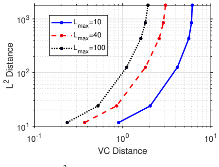
Lmin/Lmax integration bounds for IVC = e.g., Lmax = 10, 40, 100 in Fig 5.2
The IVC distance and the preprocessing criterion depend on the integration range; no criterion for choosing it is given (Definition 5.1).
KDE bandwidth for VC density = not reported
VC density and VCDR tables (Figures 3.1 and 4.6, Tables 4.1 and 4.2) are estimated by Gaussian KDE per the text, but the bandwidth is never specified, and the ratio tables with zero entries are sensitive to it.
Preprocessing threshold epsilon = unspecified
Algorithm 5.1 halts preprocessing when DistIVC <= epsilon; no value or estimation procedure is given anywhere in Section 5.3.

assumptions (4)

domain assumption f is C^1 for the derivative link between VC and slope (Proposition 3.2)
The proposition is stated only for C^1 functions, and the proof uses Taylor expansion; the claimed equality is false as stated (for f(x) = -x the LHS is 1, the RHS is -1).
standard math f is bounded on the domain so that VC is finite (Remark 3.5)
Boundedness is invoked to guarantee VC_L < infinity; standard for oscillation-type functionals, and stated by the authors.
ad hoc to paper Under translation equivalence a network only needs to approximate the shape of the objective function
Stated in Section 1 without proof; it motivates dropping constants in the IVC distance but is not established.
ad hoc to paper VC density ratio (VCDR) from KDE measurements tracks genuine approximation progress at the corresponding VC level
Used in Section 4.2 to infer the minority-tendency; contradicted by the paper's own remark in Definition 3.9 that the ratio has no reference significance near zero density.

invented entities (2)

VC (value change) functional independent evidence
purpose: Quantify local variation of the objective function to predict where neural network approximation will be accurate (Definition 3.1).
A mathematical construct equal to the classical local oscillation of f over a box; computable from function samples, so its alleged correlation with approximation error is falsifiable. Included for ledger completeness, not as a physical entity.
IVC distance independent evidence
purpose: Distance between functions used as the preprocessing criterion in Algorithm 5.1.
Defined as an integral of VC over scales and space (Definitions 5.1 and 5.2); computable, and the claim that minimizing it accelerates training is testable. Same caveat as VC: it is a repackaged classical quantity.

how reviews work

0 comments

Cite this review

Pith. "Pith review of Objective Value Change and Shape-Based Accelerated Optimization for the Neural Network Approximation." pith.science (2026). https://pith.science/paper/HJ7DQXJ4

@misc{pith2026250820290,
  author       = {Pith},
  title        = {Pith review of: Objective Value Change and Shape-Based Accelerated Optimization for the Neural Network Approximation},
  year         = {2026},
  howpublished = {\url{https://pith.science/paper/HJ7DQXJ4}},
  note         = {Machine review of arXiv:2508.20290}
}

read the original abstract

This paper introduce a novel metric of an objective function f, we say VC (value change) to measure the difficulty and approximation affection when conducting an neural network approximation task, and it numerically supports characterizing the local performance and behavior of neural network approximation. Neural networks often suffer from unpredictable local performance, which can hinder their reliability in critical applications. VC addresses this issue by providing a quantifiable measure of local value changes in network behavior, offering insights into the stability and performance for achieving the neural-network approximation. We investigate some fundamental theoretical properties of VC and identified two intriguing phenomena in neural network approximation: the VC-tendency and the minority-tendency. These trends respectively characterize how pointwise errors evolve in relation to the distribution of VC during the approximation process.In addition, we propose a novel metric based on VC, which measures the distance between two functions from the perspective of variation. Building upon this metric, we further propose a new preprocessing framework for neural network approximation. Numerical results including the real-world experiment and the PDE-related scientific problem support our discovery and pre-processing acceleration method.

Figures

Figures reproduced from arXiv: 2508.20290 by the authors.

**Figure 2.1.** Correlation between linear function slope and approximation speed/efficiency. Two threedimensional linear functions with different slopes are approximated by a neural network over [−1,1] 3 , using the Adam optimizer and mean squared error (MSE) loss. The learning rate is 10−2 [PITH_FULL_IMAGE:figures/full_fig_p004_2_1.png] view at source ↗

**Figure 2.2.** The correlation between different slopes and the approximation speed/efficiency within a single function. The optimizer is Adam and the loss is MSE. Learning rate is 10−2 [PITH_FULL_IMAGE:figures/full_fig_p005_2_2.png] view at source ↗

**Figure 3.1.** The VC Density function of (a) the piece-wise function f1, (b) the piece-wise function f2 in (2.2). The VC Density function illustrates the distribution of VC values of functions. In the case of a smooth and differentiable function, the VC value reflects the distribution of function derivatives. For example, considering a linear function f(x) = x−1, which satisfies VCL = L, the VC Density function FVCL(f,x) (VCL = L… view at source ↗

Figures from the paper (14 more)

**Figure 3.2.** Figure 3.2: (b) show the trend of pointwise error in the process of neural networks approximating f0 and f1 in (2), respectively. Figs. 3.2(a) and (b) show the total training results for the first 250 steps. In the objective functions f0 and f1, there are significant jump breaks…

**Figure 4.1.** Figure 4.1: Direct approximation of a monochrome image and VC with different diameters. (a1) Original monochrome image. (a2) Neural network approximation result. (a3) Absolute error between the approximation and the original. (b1)–(b3) VC of the original image computed with dif…

**Figure 4.2.** Figure 4.2: VC-tendency phenomenon in monochrome image approximation. (a) Point-by-point error curve sorted by VC value, and point error size distribution of different VC distribution pixels. (b1)- (b3) Correlation of error curve with VC for three different smoothing methods. To…

**Figure 4.3.** Figure 4.3: 3-dimensional VC-tendency phenomenon in the flow past a cylinder. (a): the trends of three types of errors (average, maximum, and median) for pixel points sorted according to 3-dimensional VC ordering in the flow past a cylinder, and the flipped blue area represent t…

**Figure 4.4.** Figure 4.4: Error distribution (after training) sorted by reduced order [PITH_FULL_IMAGE:figures/full_fig_p014_4_4.png]

**Figure 4.5.** Figure 4.5: Reduced order 2-dimensional VC-tendency phenomenon in the 2-dimensional flow past a cylinder. Figs. (a1)-(a3), (b1)-(b3), (c1)-(c3) respectively illustrate the correlation between three types of errors and reduced order VC at different training steps during flow past…

**Figure 4.6.** Figure 4.6: The VC Density evolution of VC when the neural networks approximate sin(2x) (left two columns) and sin(2x)+sin(6x)+sin(10x) (right two columns) by the algorithm Adam with a learning rate of 10−2 . The 1st and 3rd columns of [PITH_FULL_IMAGE:figures/full_fig_p016_4_6.png]

**Figure 5.1.** Figure 5.1: The approximation performance of different pre-training strategies. The legends A, B, and C represent the results where the neural network first approximates the intermediate objective functions g = −100x, g = 100x, and g = −10x, respectively, before subsequently app…

**Figure 5.2.** Figure 5.2: Synchronous decrease of L 2 error and VC-norm error with varying numbers of interpolation points. serves as a pre-processing model. A new neural network is then trained to approximate f − fappr, thereby indirectly approximating the original objective function. The fl…

**Figure 6.1.** Figure 6.1: Pre-processing for linear function approximation. The relation of test loss and round when adjusting the initial model and modeling f = 10x + 10y + 10z with a domain [−1,1] 3 under the logarithmic vertical axis scale. The optimizer is Adam and the loss is MSE. The le…

**Figure 6.2.** Figure 6.2: Relation of test loss and round when fitting [PITH_FULL_IMAGE:figures/full_fig_p023_6_2.png]

**Figure 6.3.** Figure 6.3: Pre-processing for image approximation. The 1st and 3rd columns show the training results of three methods for approximating monochrome pictures in two neural network settings. The other columns show the final absolute error. that the interpolation-based preprocessin…

**Figure 6.4.** Figure 6.4: The six curves represent the decreasing trend of test absolute error for three training strate [PITH_FULL_IMAGE:figures/full_fig_p025_6_4.png]

**Figure 6.5.** Figure 6.5: Approximation results across different time steps and pre-processings: rows indicate in [PITH_FULL_IMAGE:figures/full_fig_p026_6_5.png]

Review history (2 revisions) →

Discussion (0). Continue with ORCID to comment.

Reference graph

Works this paper leans on

45 extracted references · 43 canonical work pages

[1]

A LFONSI ET AL ., Reynolds averaged Navier-Stokes equations for turbulence modeling , Applied Mechanics Re- views, 63 (2009)

G. A LFONSI ET AL ., Reynolds averaged Navier-Stokes equations for turbulence modeling , Applied Mechanics Re- views, 63 (2009)

work page 2009
[2]

A. R. B ARRON , Universal approximation bounds for superpositions of a sigmoidal function , IEEE Transactions on Information Theory, 39 (1993), pp. 930–945

work page 1993
[3]

C. M. B ISHOP , Pattern recognition and machine learning, Springer, 4 (2006), pp. 738–740

work page 2006
[4]

S. C AI, Z. M AO, Z. W ANG , M. Y IN, AND G. E. K ARNIADAKIS , Physics-informed neural networks (PINNs) for fluid mechanics: A review, Acta Mechanica Sinica, 37 (2021), pp. 1727–1738

work page 2021
[5]

C ARLEO AND M

G. C ARLEO AND M. T ROYER , Solving the quantum many-body problem with artificial neural networks, Science, 355 (2017), pp. 602–606

work page 2017
[6]

R. T. Q. C HEN , Y. RUBANOVA , J. B ETTENCOURT , AND D. K. D UVENAUD , Neural ordinary differential equations, Advances in Neural Information Processing Systems, 31 (2018)

work page 2018
[7]

C YBENKO , Approximation by superpositions of a sigmoidal function , Mathematics of Control, Signals and Sys- tems, 2 (1989), pp

G. C YBENKO , Approximation by superpositions of a sigmoidal function , Mathematics of Control, Signals and Sys- tems, 2 (1989), pp. 303–314

work page 1989
[8]

G OODFELLOW , Y

I. G OODFELLOW , Y. BENGIO , A. C OURVILLE , AND Y. BENGIO , Deep learning, vol. 1, MIT press Cambridge, 2016

work page 2016

Show all 45 references

[9]

H. G UO, P. G REENGARD , E. X ING , AND Y. K IM, LQ-LoRA: Low-rank plus quantized matrix decomposition for efficient language model finetuning, in The Twelfth International Conference on Learning Representations
[10]

X. G UO, W. L I, AND F. IORIO , Convolutional neural networks for steady flow approximation, in Proceedings of the 22nd ACM SIGKDD International Conference on Knowledge Discovery and Data Mining, 2016, pp. 481–490

2016
[11]

H ORNIK , M

K. H ORNIK , M. S TINCHCOMBE , AND H. W HITE , Multilayer feedforward networks are universal approximators , Neural Networks, 2 (1989), pp. 359–366

1989
[12]

J ACOT, F

A. J ACOT, F. G ABRIEL , AND C. H ONGLER , Neural tangent kernel: Convergence and generalization in neural net- works, Advances in Neural Information Processing Systems, 31 (2018)

2018
[13]

K RIZHEVSKY , I

A. K RIZHEVSKY , I. S UTSKEVER , AND G. E. H INTON , Imagenet classification with deep convolutional neural net- works, Advances in Neural Information Processing Systems, 25 (2012)

2012
[14]

L ARSON , M

J. L ARSON , M. M ENICKELLY , AND S. M. W ILD, Derivative-free optimization methods, Acta Numerica, 28 (2019), 25 t = 0 t = 3 t = 6 t = 9 Fig. 6.5: Approximation results across different time steps and pre-processings: rows indicate in- creasing levels of pre-processing (none,...

2019
[15]

L ECUN, Y

Y. L ECUN, Y. BENGIO , AND G. H INTON , Deep learning, Nature, 521 (2015), pp. 436–444

2015
[16]

L ESHNO , V

M. L ESHNO , V. Y. L IN, A. P INKUS , AND S. S CHOCKEN , Multilayer feedforward networks with a nonpolynomial activation function can approximate any function, Neural Networks, 6 (1993), pp. 861–867

1993
[17]

C. L IU, L. Z HU, AND M. B ELKIN , On the linearity of large non-linear models: when and why the tangent kernel is constant, Advances in Neural Information Processing Systems, 33 (2020), pp. 15954–15964

2020
[18]

Z. L IU, Y. L IN, Y. C AO, H. H U, Y. W EI, Z. Z HANG , S. L IN, AND B. G UO, Swin transformer: Hierarchical vision transformer using shifted windows, in Proceedings of the IEEE/CVF International Conference on Computer Vision, 2021, pp. 10012–10022

2021
[19]

Z. L U, H. P U, F. WANG , Z. H U, AND L. WANG, The expressive power of neural networks: A view from the width , Advances in Neural Information Processing Systems, 30 (2017)

2017
[20]

P. J. M ASON , Large-eddy simulation: A critical review of the technique, Quarterly Journal of the Royal Meteorological Society, 120 (1994), pp. 1–26

1994
[21]

M NIH , K

V. M NIH , K. K AVUKCUOGLU , D. S ILVER , A. A. R USU , J. V ENESS , M. G. B ELLEMARE , A. G RAVES , M. R IED - MILLER , A. K. F IDJELAND , G. O STROVSKI , ET AL ., Human-level control through deep reinforcement learning, Nature, 518 (2015), pp. 529–533

2015
[22]

M OIN AND K

P. M OIN AND K. M AHESH , Direct numerical simulation: a tool in turbulence research , Annual Review of Fluid Mechanics, 30 (1998), pp. 539–578

1998
[23]

N O ´E, A

F. N O ´E, A. T KATCHENKO , K.-R. M ¨ULLER , AND C. C LEMENTI , Machine learning for molecular simulation, Annual Review of Physical Chemistry, 71 (2020), pp. 361–390

2020
[24]

M. J. D. P OWELL , The NEWUOA software for unconstrained optimization without derivatives , in Large-scale Non- linear Optimization, G. Pillo and M. Roma, eds., Springer, Boston, 2006, pp. 255–297

2006
[25]

R AISSI , P

M. R AISSI , P. PERDIKARIS , AND G. K ARNIADAKIS , Physics-informed neural networks: A deep learning framework for solving forward and inverse problems involving nonlinear partial differential equations, Journal of Computa- tional Physics, 378 (2019), pp. 686–707

2019
[26]

T ELGARSKY , Benefits of depth in neural networks, PMLR, 2016, pp

M. T ELGARSKY , Benefits of depth in neural networks, PMLR, 2016, pp. 1517–1539

2016
[27]

T REBOTICH AND D

D. T REBOTICH AND D. G RAVES, An adaptive finite volume method for the incompressible Navier–Stokes equations in 26 complex geometries, Communications in Applied Mathematics and Computational Science, 10 (2015), pp. 43–82

2015
[28]

W ANG , S

S. W ANG , S. S ANKARAN , P. S TINIS , AND P. PERDIKARIS , Simulating three-dimensional turbulence with physics- informed neural networks, arXiv preprint arXiv:2507.08972, (2025)

2025
[29]

W ANG , X

S. W ANG , X. Y U, AND P. P ERDIKARIS , When and why PINNs fail to train: A neural tangent kernel perspective , Journal of Computational Physics, 449 (2022), p. 110768

2022
[30]

S. M. W ILD , R. G. R EGIS , AND C. A. S HOEMAKER , ORBIT: Optimization by radial basis function interpolation in trust-regions, SIAM Journal on Scientific Computing, 30 (2008), pp. 3197–3219

2008
[31]

F. W U, Z. L I, Y. L I, B. D ING , AND J. G AO, Fedbiot: LLM local fine-tuning in federated learning without full model, in Proceedings of the 30th ACM SIGKDD Conference on Knowledge Discovery and Data Mining, 2024, pp. 3345–3355

2024
[32]

P. X IE, Sufficient conditions for error distance reduction in the ℓ2-norm trust region between minimizers of local nonconvex multivariate quadratic approximates, Journal of Computational and Applied Mathematics, 453 (2025), p. 116146

2025
[33]

X IE AND S

P. X IE AND S. M. W ILD, ReMU: Regional minimal updating for model-based derivative-free optimization , 2025, https://arxiv.org/abs/2504.03606

2025 arXiv
[34]

X IE AND Y

P. X IE AND Y. YUAN, A derivative-free optimization algorithm combining line-search and trust-region techniques , Chinese Annals of Mathematics, Series B, 44 (2023), pp. 719–734

2023
[35]

X IE AND Y

P. X IE AND Y. YUAN, Derivative-free optimization with transformed objective functions and the algorithm based on the least Frobenius norm updating quadratic model , Journal of the Operations Research Society of China, 13 (2025), pp. 327–363

2025
[36]

X IE AND Y

P. X IE AND Y. Y UAN, Least H 2 norm updating of quadratic interpolation models for derivative-free trust-region algorithms, IMA Journal of Numerical Analysis, (2025), p. drae106

2025
[37]

X IE AND Y.-X

P. X IE AND Y.-X. Y UAN, A derivative-free method using a new underdetermined quadratic interpolation model , SIAM Journal on Optimization, 35 (2025), pp. 1110–1133

2025
[38]

X IE AND J

T. X IE AND J. C. G ROSSMAN , Crystal graph convolutional neural networks for an accurate and interpretable pre- diction of material properties, Physical Review Letters, 120 (2018), p. 145301

2018
[39]

Z.-Q. J. X U, Y. ZHANG , AND T. LUO, Overview frequency principle/spectral bias in deep learning, Communications on Applied Mathematics and Computation, (2024), pp. 1–38

2024
[40]

Z.-Q. J. X U, Y. Z HANG , AND Y. XIAO, Frequency principle: Fourier analysis sheds light on deep neural networks, Communications in Computational Physics, 28 (2020), pp. 1746–1767

2020
[41]

Y ANG , F

S. Y ANG , F. Z HAO, Z. Z HOU , L. S HI, X. R EN, AND Z. X U, Review of mathematical optimization in federated learning, arXiv preprint arXiv:2412.01630, (2024)

2024 arXiv
[42]

Y ANG , R

Y. Y ANG , R. K HANNA , Y. Y U, A. G HOLAMI , K. K EUTZER , J. E. G ONZALEZ , K. R AMCHANDRAN , AND M. W. MAHONEY , Boundary thickness and robustness in learning models , vol. 33, Curran Associates, Inc., 2020, pp. 6223–6234

2020
[43]

Y AROTSKY , Error bounds for approximations with deep ReLU networks , Neural Networks, 94 (2017), pp

D. Y AROTSKY , Error bounds for approximations with deep ReLU networks , Neural Networks, 94 (2017), pp. 103– 114

2017
[44]

Z HOU , Y

Z. Z HOU , Y. L I, X. R EN, AND S. Y ANG, Towards efficient and stable K-asynchronous federated learning with unbounded stale gradients on non-iid data , IEEE Transactions on Parallel and Distributed Systems, 33 (2022), pp. 3291–3305

2022
[45]

Z HOU AND Z

Z. Z HOU AND Z. Y AN, Is the neural tangent kernel of PINNs deep learning general partial differential equations always convergent?, Physica D: Nonlinear Phenomena, 457 (2024), p. 133987. 27

2024

Pith tools

Reviewed August 15, 2026 · model on record in the stance chip above.

[1] [1]

A LFONSI ET AL ., Reynolds averaged Navier-Stokes equations for turbulence modeling , Applied Mechanics Re- views, 63 (2009)

G. A LFONSI ET AL ., Reynolds averaged Navier-Stokes equations for turbulence modeling , Applied Mechanics Re- views, 63 (2009)

work page 2009

[2] [2]

A. R. B ARRON , Universal approximation bounds for superpositions of a sigmoidal function , IEEE Transactions on Information Theory, 39 (1993), pp. 930–945

work page 1993

[3] [3]

C. M. B ISHOP , Pattern recognition and machine learning, Springer, 4 (2006), pp. 738–740

work page 2006

[4] [4]

S. C AI, Z. M AO, Z. W ANG , M. Y IN, AND G. E. K ARNIADAKIS , Physics-informed neural networks (PINNs) for fluid mechanics: A review, Acta Mechanica Sinica, 37 (2021), pp. 1727–1738

work page 2021

[5] [5]

C ARLEO AND M

G. C ARLEO AND M. T ROYER , Solving the quantum many-body problem with artificial neural networks, Science, 355 (2017), pp. 602–606

work page 2017

[6] [6]

R. T. Q. C HEN , Y. RUBANOVA , J. B ETTENCOURT , AND D. K. D UVENAUD , Neural ordinary differential equations, Advances in Neural Information Processing Systems, 31 (2018)

work page 2018

[7] [7]

C YBENKO , Approximation by superpositions of a sigmoidal function , Mathematics of Control, Signals and Sys- tems, 2 (1989), pp

G. C YBENKO , Approximation by superpositions of a sigmoidal function , Mathematics of Control, Signals and Sys- tems, 2 (1989), pp. 303–314

work page 1989

[8] [8]

G OODFELLOW , Y

I. G OODFELLOW , Y. BENGIO , A. C OURVILLE , AND Y. BENGIO , Deep learning, vol. 1, MIT press Cambridge, 2016

work page 2016