arxiv: 2508.21216 · v2 · submitted 2025-08-28 · 🌀 gr-qc

Persistence of post-Newtonian amplitude structure in binary black hole mergers

Viviana A. C\'aceres-Barbosa This is my paper

Pith reviewed 2026-05-18 20:07 UTC · model grok-4.3

classification 🌀 gr-qc

keywords binary black holesgravitational wave modespost-Newtonian approximationnumerical relativitywaveform amplitudesmass ratio dependencemerger phase

0 comments p. Extension

The pith

Certain binary black hole waveform modes retain leading post-Newtonian mass ratio dependence through merger.

A machine-rendered reading of the paper's core claim, the machinery that carries it, and where it could break.

The paper examines spherical harmonic mode amplitudes in quasicircular nonprecessing binary black hole mergers drawn from 275 numerical relativity simulations. It tests how well leading-order post-Newtonian expressions for amplitude dependence on mass ratio and spin continue to describe the signals when the merger occurs. For nonspinning cases the (2,2), (2,1) and (3,3) modes keep this dependence from late inspiral through postmerger. Higher modes deviate only near and after merger and are captured by adding low-degree polynomial corrections in mass ratio. The approach yields closed-form expressions that link weak-field and strong-field regimes for efficient waveform modeling.

Core claim

For nonspinning systems the (2,2), (2,1), and (3,3) modes retain the leading-order PN dependence on mass ratio throughout the merger. Higher-order modes deviate from the PN dependence only near and after the merger, where polynomial fits of degree N ≤ 3 can capture the amplitude behavior up to 40M. For aligned-spin systems at fixed mass ratio the (2,1) mode retains its PN spin dependence while the (3,2) and (4,3) modes exhibit a quadratic spin dependence near merger.

What carries the argument

Leading-order post-Newtonian amplitude Ansatz with the velocity term replaced by fitted coefficients and supplemented by low-degree polynomial corrections in mass ratio and spin.

If this is right

PN-inspired fits lose accuracy with increasing mass ratio especially near merger.
Polynomial fits of degree N ≤ 3 describe higher-mode amplitudes up to 40M after the (2,2) peak.
The (2,1) mode keeps its PN spin dependence while (3,2) and (4,3) show quadratic spin dependence near merger.
Results are broadly consistent across catalogs though some modes show resolution-related differences.

Where Pith is reading between the lines

These are editorial extensions of the paper, not claims the author makes directly.

The same PN-plus-polynomial form could be tested on precessing binaries to check whether the persistence generalizes.
Hybrid inspiral-merger models might match PN waveforms to NR data with fewer free parameters by using these corrections.
Catalog discrepancies in higher modes suggest that resolution studies focused on (3,1) and (4,1) would be useful.
Closed-form amplitude expressions of this type could speed up surrogate waveform generation for data analysis.

Load-bearing premise

The leading-order post-Newtonian dependence on intrinsic parameters supplies a functional form for mode amplitudes that can be corrected by low-degree polynomials to cover late inspiral through postmerger.

What would settle it

New simulations at high mass ratio where the (2,2) mode amplitude near merger deviates strongly from the fitted leading-order PN form would falsify the persistence claim.

Figures

Figures reproduced from arXiv: 2508.21216 by Viviana A. C\'aceres-Barbosa.

**Figure 2.** Figure 2: FIG. 2 [PITH_FULL_IMAGE:figures/full_fig_p007_2.png] view at source ↗

**Figure 3.** Figure 3: FIG. 3 [PITH_FULL_IMAGE:figures/full_fig_p008_3.png] view at source ↗

**Figure 4.** Figure 4: FIG. 4 [PITH_FULL_IMAGE:figures/full_fig_p009_4.png] view at source ↗

**Figure 5.** Figure 5: FIG. 5 [PITH_FULL_IMAGE:figures/full_fig_p010_5.png] view at source ↗

**Figure 6.** Figure 6: FIG. 6 [PITH_FULL_IMAGE:figures/full_fig_p011_6.png] view at source ↗

**Figure 7.** Figure 7: FIG. 7 [PITH_FULL_IMAGE:figures/full_fig_p015_7.png] view at source ↗

**Figure 8.** Figure 8: FIG. 8 [PITH_FULL_IMAGE:figures/full_fig_p016_8.png] view at source ↗

**Figure 9.** Figure 9: FIG. 9 [PITH_FULL_IMAGE:figures/full_fig_p017_9.png] view at source ↗

read the original abstract

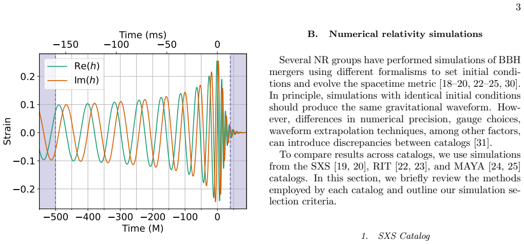
We analyze the spherical harmonic mode amplitudes of quasicircular, nonprecessing binary black hole mergers using 275 numerical relativity simulations from the SXS, RIT, and MAYA catalogs. We construct fits using the leading-order post-Newtonian (PN) dependence on intrinsic parameters, replacing the PN velocity with fit coefficients. We compare these to polynomial fits in symmetric mass ratio and spin. We analyze $(\ell, m)$ modes with $\ell \leq 4$ from late inspiral [$t = -500M$ relative to the $(2,2)$ peak] to postmerger ($t = 40M$). For nonspinning systems, the $(2,2)$, $(2,1)$, and $(3,3)$ modes retain the leading-order PN dependence on mass ratio throughout the merger. Higher-order modes deviate from the PN dependence only near and after the merger, where polynomial fits of degree $N \leq 3$ can capture the amplitude behavior up to $40M$. For aligned-spin systems at fixed mass ratio, the $(2,1)$ mode retains its PN spin dependence, while the $(3,2)$ and $(4,3)$ modes exhibit a quadratic spin dependence near merger. The PN-inspired fits lose accuracy with increasing mass ratio, particularly near merger. Results broadly agree across catalogs, though discrepancies appear in the $(3,1)$, $(4,2)$, and $(4,1)$ modes, likely from resolution differences. Our results clarify the extent to which PN structure persists in mode amplitudes. Although the fits cannot be fully interpreted within the PN formalism near merger, low-degree polynomial corrections to the PN amplitude Ans\"atze can capture strong-field behavior, enabling closed-form and efficient modeling of waveform amplitudes in this regime.

Editorial analysis

A structured set of objections, weighed in public.

Desk editor's note, referee report, simulated authors' rebuttal, and a circularity audit. Tearing a paper down is the easy half of reading it; the pith above is the substance, this is the friction.

Desk Editor's Note private letter to a colleague

The paper shows that leading PN mass-ratio dependence holds through merger for the (2,2), (2,1), and (3,3) modes in nonspinning cases, with low-degree polynomials handling the rest, from fits to 275 simulations.

read the letter

The main point is that for nonspinning binary black hole mergers the (2,2), (2,1), and (3,3) mode amplitudes keep the leading-order post-Newtonian mass-ratio dependence all the way through merger when the velocity factor is replaced by a fitted coefficient. Higher modes only need low-degree polynomial corrections near and after merger. The aligned-spin runs at fixed mass ratio show the (2,1) mode retaining its PN spin dependence while (3,2) and (4,3) pick up quadratic spin terms near merger. The work draws on 275 simulations from the SXS, RIT, and MAYA catalogs and tracks amplitudes from t = -500M to +40M relative to the (2,2) peak. It directly compares the PN-inspired fits against pure polynomial fits in symmetric mass ratio and spin, which gives a clear picture of where the PN form still adds something useful. The sample size and multi-catalog check are the strongest parts; the results line up across catalogs for the low modes and the authors flag the loss of accuracy at higher mass ratios. The soft spots are the drop in fit quality with increasing mass ratio, especially near merger, and the catalog differences in a few higher modes that get attributed to resolution. Those points limit how far the persistence claim can be pushed without more resolution studies. The method is empirical fitting rather than a derivation, so the results document what works in the data rather than proving why. This is the sort of targeted check that waveform modelers will use when they want simple closed-form amplitude pieces that reach into the strong-field regime. Readers building efficient models for gravitational-wave data analysis will get the most from the mode-by-mode findings. It is solid enough to deserve a serious referee because the dataset is large, the claims are specific, and the comparison to polynomials is straightforward to evaluate.

Referee Report

2 major / 2 minor

Summary. The paper analyzes spherical harmonic mode amplitudes of quasicircular, nonprecessing binary black hole mergers using 275 numerical relativity simulations from the SXS, RIT, and MAYA catalogs. It constructs fits based on the leading-order post-Newtonian (PN) dependence on intrinsic parameters, replacing the PN velocity term with fitted coefficients, and compares these to polynomial fits in symmetric mass ratio and spin. Modes with ℓ ≤ 4 are examined from late inspiral (t = -500M relative to the (2,2) peak) to postmerger (t = 40M). For nonspinning systems, the (2,2), (2,1), and (3,3) modes retain the leading-order PN mass-ratio dependence throughout the merger, while higher-order modes deviate only near and after merger where low-degree (N ≤ 3) polynomials suffice. For aligned-spin systems at fixed mass ratio, the (2,1) mode retains PN spin dependence and the (3,2), (4,3) modes show quadratic spin dependence near merger. PN-inspired fits lose accuracy at high mass ratio, with broad agreement across catalogs except for some higher modes attributed to resolution differences.

Significance. If the central empirical findings hold, the work shows that PN-inspired ansatze with modest low-degree polynomial corrections can describe mode amplitudes from late inspiral through postmerger, offering a route to closed-form, efficient amplitude modeling in the strong-field regime. The multi-catalog analysis with 275 simulations, explicit time ranges, and direct comparison of PN-inspired versus polynomial forms provides a concrete, falsifiable basis for the persistence claim. This is a useful bridge between PN theory and NR data for gravitational-wave waveform construction.

major comments (2)

[Fitting procedure and results sections] The central claim that the (2,2), (2,1), and (3,3) modes retain leading-order PN mass-ratio dependence rests on replacing the PN velocity term with fitted coefficients, yet the manuscript provides no explicit functional form for the ansatz, no equation for the coefficient optimization, and no description of the data selection or error weighting used in the fits. This detail is load-bearing for assessing whether the reported persistence is robust or an artifact of the fitting procedure.
[Results for higher-order modes] The statement that polynomial fits of degree N ≤ 3 capture the amplitude behavior up to t = +40M for higher-order modes is presented without specifying the exact polynomial basis, the fitting interval boundaries, or quantitative goodness-of-fit metrics (e.g., residuals or reduced χ²) across the catalogs. This undermines evaluation of the post-merger modeling claim.

minor comments (2)

[Analysis setup] The time coordinate is stated as t = -500M relative to the (2,2) peak, but it is unclear whether this reference time is identical for all modes or adjusted per mode; a brief clarification would improve reproducibility.
[Catalog comparison] Discrepancies in the (3,1), (4,2), and (4,1) modes are attributed to resolution differences, but no quantitative convergence test or resolution comparison table is referenced; adding such a table would strengthen the catalog-agreement claim.

Simulated Author's Rebuttal

2 responses · 0 unresolved

We thank the referee for their careful reading of the manuscript and for identifying points where additional methodological detail will strengthen the presentation. We address each major comment below and have revised the manuscript to incorporate the requested clarifications.

read point-by-point responses

Referee: [Fitting procedure and results sections] The central claim that the (2,2), (2,1), and (3,3) modes retain leading-order PN mass-ratio dependence rests on replacing the PN velocity term with fitted coefficients, yet the manuscript provides no explicit functional form for the ansatz, no equation for the coefficient optimization, and no description of the data selection or error weighting used in the fits. This detail is load-bearing for assessing whether the reported persistence is robust or an artifact of the fitting procedure.

Authors: We agree that the fitting procedure was described too briefly. In the revised manuscript we have added an explicit subsection that states the functional form of the PN-inspired ansatz (replacing the leading PN velocity factor with a time-dependent coefficient while preserving the exact mass-ratio prefactor from leading-order PN), the least-squares optimization equation used to determine the coefficients, the data-selection criteria (all 275 simulations with mass ratios up to 10 and dimensionless spins up to 0.8), and the uniform weighting applied after normalizing each mode amplitude by its value at t = -500M. These additions make the procedure fully reproducible and allow direct assessment that the reported persistence is not an artifact of the fit. revision: yes
Referee: [Results for higher-order modes] The statement that polynomial fits of degree N ≤ 3 capture the amplitude behavior up to t = +40M for higher-order modes is presented without specifying the exact polynomial basis, the fitting interval boundaries, or quantitative goodness-of-fit metrics (e.g., residuals or reduced χ²) across the catalogs. This undermines evaluation of the post-merger modeling claim.

Authors: We accept that quantitative detail was omitted. The revised text now specifies that the polynomials are written in the monomial basis of the symmetric mass ratio η (i.e., ∑_{k=0}^N a_k η^k with N ≤ 3), that the fits are performed over the fixed interval t ∈ [-500M, +40M] relative to the (2,2) peak, and that we report reduced-χ² values and maximum residuals for each mode and each catalog. These metrics confirm that N ≤ 3 yields residuals consistent with numerical noise for the higher modes after merger, thereby supporting the post-merger modeling claim. revision: yes

Circularity Check

0 steps flagged

No significant circularity

full rationale

The paper performs an empirical analysis of 275 numerical relativity simulations from external catalogs (SXS, RIT, MAYA). It constructs phenomenological fits by adopting the leading-order PN functional form for mode amplitudes as an ansatz, replacing the velocity factor with coefficients fitted directly to the simulation data, then compares these to low-degree polynomial fits in mass ratio and spin. The central claim is an observational statement about the persistence of that functional form in the data for specific modes up to t = +40M, with explicit discussion of where it deviates and where polynomial corrections suffice. No derivation reduces to its own inputs by construction, no load-bearing self-citation chain is invoked, and the reported findings are falsifiable against the simulation data rather than tautological. This is a standard data-driven modeling study with no circularity in the claimed results.

Axiom & Free-Parameter Ledger

1 free parameters · 1 axioms · 0 invented entities

The analysis rests on treating leading-order PN forms as a useful starting Ansatz for amplitudes and on the assumption that the three simulation catalogs provide sufficiently accurate and representative data for drawing conclusions about mode behavior.

free parameters (1)

fit coefficients replacing PN velocity term
Coefficients are introduced to replace the post-Newtonian velocity in the amplitude Ansatz and are determined by fitting to the numerical relativity data.

axioms (1)

domain assumption Leading-order post-Newtonian dependence on intrinsic parameters is a valid starting Ansatz for spherical harmonic mode amplitudes
This premise is used to construct the PN-inspired fits that are then compared to polynomial fits and to the simulation data.

pith-pipeline@v0.9.0 · 5855 in / 1701 out tokens · 88248 ms · 2026-05-18T20:07:20.042709+00:00 · methodology

discussion (0)

Lean theorems connected to this paper

Citations machine-checked in the Pith Canon. Every link opens the source theorem in the public Lean library.

IndisputableMonolith/Foundation/RealityFromDistinction.lean reality_from_one_distinction unclear

?

unclear
Relation between the paper passage and the cited Recognition theorem.

We construct fits using the leading-order post-Newtonian (PN) dependence on intrinsic parameters, replacing the PN velocity with fit coefficients... polynomial fits of degree N ≤ 3 can capture the amplitude behavior up to 40M.

What do these tags mean?

matches: The paper's claim is directly supported by a theorem in the formal canon.
supports: The theorem supports part of the paper's argument, but the paper may add assumptions or extra steps.
extends: The paper goes beyond the formal theorem; the theorem is a base layer rather than the whole result.
uses: The paper appears to rely on the theorem as machinery.
contradicts: The paper's claim conflicts with a theorem or certificate in the canon.
unclear: Pith found a possible connection, but the passage is too broad, indirect, or ambiguous to say the theorem truly supports the claim.

Reference graph

Works this paper leans on

71 extracted references · 71 canonical work pages · 26 internal anchors

[1]

SXS Catalog The SXS catalog utilizes the Spectral Einstein Code

work page
[2]

The initial data is generated by solving the extended conformal thin-sandwich equa- tions, which are discretized on a grid and solved using a spectral elliptic solver

to perform simulations. The initial data is generated by solving the extended conformal thin-sandwich equa- tions, which are discretized on a grid and solved using a spectral elliptic solver. Iterative tuning is applied to achieve the desired BBH properties, and the initial data is evolved for several orbits to reduce eccentricity and produce quasi-circul...

work page
[3]

RIT Catalog The simulations in the RIT catalog are generated using the LazEv code [38]. The initial data for RIT simula- tions is derived from the Bowen-York solution and com- puted using a generalized version of theTwoPunctures code [39], which solves a coupled system of the Hamil- tonian and momentum constraints. RIT simulations use PN approximations [4...

work page
[4]

Each simulation has a resolution labeled nXYY, where the grid spacing of the refinement level at which the waveform is extracted is specified as M/X.Y Y

infrastructure from the EinsteinToolkit [45] and 4 uses the Carpet [46] module for mesh refinement. Each simulation has a resolution labeled nXYY, where the grid spacing of the refinement level at which the waveform is extracted is specified as M/X.Y Y . For example, n120 corresponds to a grid spacing of M/1.2. Only simulations with a resolution label of ...

work page
[5]

Similar to LazEv, the MAYA code uses the Cactus/Carpet/EinsteinToolkit infrastructure for its simulations

MAYA Catalog The simulations in the MAYA catalog use the MAYA code [25]. Similar to LazEv, the MAYA code uses the Cactus/Carpet/EinsteinToolkit infrastructure for its simulations. It constructs initial data based on the Bowen-York extrinsic curvature, conformally flat spatial metric, and the TwoPunctures solver. The PN equa- tions of motion are also used ...

work page
[6]

Additionally, all simulations are selected to have initial orbital eccentricities of less than 0.002, as reported by their respective catalogs

Selection criteria The linear shift in the time origin of the coordinates, which arises from the residual motion of the center of mass of the binary system [50], was corrected for all sim- ulations used. Additionally, all simulations are selected to have initial orbital eccentricities of less than 0.002, as reported by their respective catalogs. 4 For non...

work page
[7]

(7i) (7j) To perform the fits, we extract ˆAℓm from the NR simu- lation at each time step and apply the fitting functions presented above

Leading-order fits for nonspinning simulations For nonspinning simulations, the resulting leading- order fitting functions are: ˆA(LO) 22 = 8 r π 5 η a(2) 22 , (7a) ˆA(LO) 21 = 1 3 δ a(1) 21 , (7b) ˆA(LO) 33 = 3 4 r 15 14 δ a(1) 33 , (7c) ˆA(LO) 32 = 1 3 r 5 7 (1 − 3η) a(2) 32 , (7d) ˆA(LO) 31 = δ 12 √ 14 a(1) 31 , (7e) ˆA(LO) 44 = −8 9 r 5 7(3η − 1)a(2) ...

work page
[8]

(8d) where ˆAns ℓm is the ( ℓ, m) mode amplitude of a nonspin- ning system with the corresponding mass ratio

Leading-order fits for aligned-spin simulations For aligned-spin systems, the resulting fits are: ˆA(LO,S) 21 = ˆAns 21 − 1 2 (χa + δχs) a(2) 21 , (8a) ˆA(LO,S) 32 = ˆAns 32 + 4 3 r 5 7 ηχsa(3) 32 , (8b) ˆA(LO,S) 43 = ˆAns 43 + 45 8 √ 70 η (χa − δχs) a(4) 43 , (8c) ˆA(LO,S) 41 = ˆAns 41 + 5 84 √ 40 η (δχs − χa) a(4) 41 . (8d) where ˆAns ℓm is the ( ℓ, m) ...

work page
[9]

Our primary focus in this section is on the quality of the fit, rather than the physical interpretation of the coef- ficients

Higher-order fits for nonspinning simulations We construct fitting functions for the relative mode amplitudes of nonspinning systems that incorporate higher-order dependencies on the symmetric mass ratio η. Our primary focus in this section is on the quality of the fit, rather than the physical interpretation of the coef- ficients. Therefore, we do not ex...

work page
[10]

(10b) As done with the leading-order fits, we fix the mass ratio and use the nonspinning NR reference amplitudes ˆAns ℓm

Higher-order fits for aligned-spin simulations Similarly, for aligned-spin systems, we define higher- order fitting functions that incorporate linear and quadratic dependencies on χs and χa: ˆA(1,S) ℓm = ˆAns ℓm + X i=a,s ciχi, (10a) ˆA(2,S) ℓm = ˆAns ℓm + X i=a,s ciχi + X i=a,s X j=a,s cijχiχj. (10b) As done with the leading-order fits, we fix the mass r...

work page
[11]

2 shows the optimal fit parameters obtained for the leading-order models defined in Eqs

Nonspinning simulations Fig. 2 shows the optimal fit parameters obtained for the leading-order models defined in Eqs. 7 over the time interval considered, using individual catalogs and the joint dataset. To directly compare the fit coefficients, the figure shows n q a(n) ℓm, so that all parameters correspond to fitting for v at early times. The Pearson co...

work page
[12]

Aligned-spin simulations To reduce the impact of cross-catalog differences, we performed fits on the aligned-spin simulations using only 7 FIG. 2. Leading-order fits for nonspinning simulations : Optimal fit coefficients n q a(n) ℓm and Pearson correlation Cℓm for the leading-order fits defined in Eqs. 7, shown as a function of time t after the peak of th...

work page
[13]

Nonspinning simulations The impact of higher-order corrections on the quality of fits for nonspinning systems is illustrated in two com- plementary figures. Fig. 4 shows the Pearson correlation coefficients for each mode obtained when applying fits of different degrees N, while Fig. 5 provides snapshots of the amplitude data and their corresponding fits a...

work page
[14]

6 shows the Pearson correlation of the higher- order aligned-spin fits ˆA(i,S) lm defined in Eq

Aligned-spin simulations Fig. 6 shows the Pearson correlation of the higher- order aligned-spin fits ˆA(i,S) lm defined in Eq. 10 for each mode across time, with the corresponding values from the leading-order fits included for reference. To further illustrate the behavior of the fits, Figs. 7–9 present snap- shots of the amplitude data and their associat...

work page 2093
[15]

(LIGO Instrument Science Collaboration) 2025 Class

S. Soni et al. (LIGO), Class. Quant. Grav. 42, 085016 (2025), arXiv:2409.02831 [astro-ph.IM]

work page arXiv 2025
[16]

Advanced LIGO

J. Aasi et al. (LIGO Scientific), Class. Quant. Grav. 32, 074001 (2015), arXiv:1411.4547 [gr-qc]. 15 1.0 0.5 0.0 0.5 1.0 1z 1.0 0.5 0.00.51.0 2z 0.00 0.50 1.00 1.50 2.00 A21 [×10 1] t = 8.84M Leading Order Quadratic 1.0 0.5 0.0 0.5 1.0 1z 1.0 0.5 0.00.51.0 2z 0.00 0.50 1.00 1.50 2.00 A21 [×10 1] t = 0.70M Leading Order Quadratic 1.0 0.5 0.0 0.5 1.0 1z 1.0...

work page internal anchor Pith review Pith/arXiv arXiv 2015
[17]

Advanced Virgo: a 2nd generation interferometric gravitational wave detector

F. Acernese et al. (VIRGO), Class. Quant. Grav. 32, 024001 (2015), arXiv:1408.3978 [gr-qc]

work page internal anchor Pith review Pith/arXiv arXiv 2015
[18]

Akutsuet al.(KAGRA), Prog

T. Akutsu et al. (KAGRA), PTEP 2021, 05A101 (2021), arXiv:2005.05574 [physics.ins-det]

work page arXiv 2021
[19]

Numerical Relativity and Astrophysics

L. Lehner and F. Pretorius, Ann. Rev. Astron. Astro- phys. 52, 661 (2014), arXiv:1405.4840 [astro-ph.HE]

work page internal anchor Pith review Pith/arXiv arXiv 2014
[20]

Post-Newtonian Theory for Gravitational Waves

L. Blanchet, Living Rev. Rel. 17, 2 (2014), arXiv:1310.1528 [gr-qc]

work page internal anchor Pith review Pith/arXiv arXiv 2014
[21]

Quasinormal modes of black holes and black branes

E. Berti, V. Cardoso, and A. O. Starinets, Class. Quant. Grav. 26, 163001 (2009), arXiv:0905.2975 [gr-qc]

work page internal anchor Pith review Pith/arXiv arXiv 2009
[22]

B. J. Kelly and J. G. Baker, Phys. Rev. D 87, 084004 (2013), arXiv:1212.5553 [gr-qc]

work page internal anchor Pith review Pith/arXiv arXiv 2013
[23]

Abbott et al

R. Abbott et al. (LIGO Scientific, Virgo), Phys. Rev. Lett. 125, 101102 (2020), arXiv:2009.01075 [gr-qc]

work page arXiv 2020
[24]

A. G. Abac et al. (LIGO Scientific, VIRGO, KAGRA), (2025), arXiv:2507.08219 [astro-ph.HE]

work page internal anchor Pith review Pith/arXiv arXiv 2025
[25]

Borhanian, K

S. Borhanian, K. G. Arun, H. P. Pfeiffer, and B. S. Sathyaprakash, Class. Quant. Grav. 37, 065006 (2020), arXiv:1901.08516 [gr-qc]

work page arXiv 2020
[26]

Is black-hole ringdown a memory of its progenitor?

I. Kamaretsos, M. Hannam, and B. Sathyaprakash, Phys. Rev. Lett. 109, 141102 (2012), arXiv:1207.0399 [gr-qc]

work page internal anchor Pith review Pith/arXiv arXiv 2012
[27]

Black-hole hair loss: learning about binary progenitors from ringdown signals

I. Kamaretsos, M. Hannam, S. Husa, and B. S. Sathyaprakash, Phys. Rev. D 85, 024018 (2012), arXiv:1107.0854 [gr-qc]

work page internal anchor Pith review Pith/arXiv arXiv 2012
[28]

Islam, (2024), arXiv:2403.03487 [gr-qc]

T. Islam, (2024), arXiv:2403.03487 [gr-qc]

work page arXiv 2024
[29]

Nobili, S

F. Nobili, S. Bhagwat, C. Pacilio, and D. Gerosa, Phys. Rev. D 112, 044058 (2025), arXiv:2504.17021 [gr-qc]

work page arXiv 2025
[30]

Pacilio, S

C. Pacilio, S. Bhagwat, F. Nobili, and D. Gerosa, Phys. Rev. D 110, 103037 (2024), arXiv:2408.05276 [gr-qc]

work page arXiv 2024
[31]

Modeling Ringdown: Beyond the Fundamental Quasi-Normal Modes

L. London, D. Shoemaker, and J. Healy, Phys. Rev. D 90, 124032 (2014), [Erratum: Phys.Rev.D 94, 069902 (2016)], arXiv:1404.3197 [gr-qc]

work page internal anchor Pith review Pith/arXiv arXiv 2014
[32]

Calibration of Moving Puncture Simulations

B. Bruegmann, J. A. Gonzalez, M. Hannam, S. Husa, U. Sperhake, and W. Tichy, Phys. Rev. D 77, 024027 (2008), arXiv:gr-qc/0610128

work page internal anchor Pith review Pith/arXiv arXiv 2008
[33]

M. A. Scheel et al., (2025), arXiv:2505.13378 [gr-qc]

work page arXiv 2025
[34]

Boyle et al., Class

M. Boyle et al., Class. Quant. Grav. 36, 195006 (2019), arXiv:1904.04831 [gr-qc]

work page arXiv 2019
[35]

Carullo, JCAP 10, 061, arXiv:2406.19442 [gr-qc]

G. Carullo, JCAP 10, 061, arXiv:2406.19442 [gr-qc]

work page arXiv
[36]

The nonspinning binary black hole merger scenario revisited

J. Healy, C. O. Lousto, and Y. Zlochower, Phys. Rev. D 96, 024031 (2017), arXiv:1705.07034 [gr-qc]

work page internal anchor Pith review Pith/arXiv arXiv 2017
[37]

Healy and C

J. Healy and C. O. Lousto, Phys. Rev. D 102, 104018 (2020), arXiv:2007.07910 [gr-qc]

work page arXiv 2020
[38]

K. Jani, J. Healy, J. A. Clark, L. London, P. Laguna, and D. Shoemaker, Class. Quant. Grav. 33, 204001 (2016), arXiv:1605.03204 [gr-qc]

work page internal anchor Pith review Pith/arXiv arXiv 2016
[39]

Ferguson et al

D. Ferguson et al. , Phys. Rev. D 112, 044043 (2025), arXiv:2309.00262 [gr-qc]

work page arXiv 2025
[40]

K. S. Thorne, Rev. Mod. Phys. 52, 299 (1980)

work page 1980
[41]

L. E. Kidder, Phys. Rev. D 77, 044016 (2008), arXiv:0710.0614 [gr-qc]

work page internal anchor Pith review Pith/arXiv arXiv 2008
[42]

C. K. Mishra, A. Kela, K. G. Arun, and G. Faye, Phys. Rev. D 93, 084054 (2016), arXiv:1601.05588 [gr-qc]

work page internal anchor Pith review Pith/arXiv arXiv 2016
[43]

B. P. Abbott et al. (LIGO Scientific, Virgo), Phys. Rev. Lett. 116, 061102 (2016), arXiv:1602.03837 [gr-qc]

work page internal anchor Pith review Pith/arXiv arXiv 2016
[44]

S. Husa, J. A. Gonzalez, M. Hannam, B. Bruegmann, and U. Sperhake, Class. Quant. Grav. 25, 105006 (2008), arXiv:0706.0740 [gr-qc]

work page internal anchor Pith review Pith/arXiv arXiv 2008
[45]

Modeling the source of GW150914 with targeted numerical-relativity simulations

G. Lovelace et al., Class. Quant. Grav.33, 244002 (2016), arXiv:1607.05377 [gr-qc]

work page internal anchor Pith review Pith/arXiv arXiv 2016
[46]

SpEC: Spectral Einstein Code — black-holes.org, https: //www.black-holes.org/code/SpEC.html

work page
[47]

Friedrich, Commun

H. Friedrich, Commun. Math. Phys. 100, 525 (1985)

work page 1985
[48]

Garfinkle, Phys

D. Garfinkle, Phys. Rev. D 65, 044029 (2002), arXiv:gr- qc/0110013

work page arXiv 2002
[49]

Numerical Relativity Using a Generalized Harmonic Decomposition

F. Pretorius, Class. Quant. Grav. 22, 425 (2005), arXiv:gr-qc/0407110

work page internal anchor Pith review Pith/arXiv arXiv 2005
[50]

Boyle, K

M. Boyle, K. Mitman, M. Scheel, and L. Stein, The sxs package (2025)

work page 2025
[51]

SXS Collaboration, The sxs catalog of simulations v3.0.0 (2025)

work page 2025
[52]

Zlochower, J

Y. Zlochower, J. G. Baker, M. Campanelli, and C. O. Lousto, Phys. Rev. D 72, 024021 (2005), arXiv:gr- qc/0505055

work page arXiv 2005
[53]

A single-domain spectral method for black hole puncture data

M. Ansorg, B. Bruegmann, and W. Tichy, Phys. Rev. D 70, 064011 (2004), arXiv:gr-qc/0404056

work page internal anchor Pith review Pith/arXiv arXiv 2004
[54]

Healy, C

J. Healy, C. O. Lousto, H. Nakano, and Y. Zlochower, Class. Quant. Grav. 34, 145011 (2017), [Erratum: Class.Quant.Grav. 40, 249502 (2023)], arXiv:1702.00872 [gr-qc]

work page arXiv 2017
[55]

T. W. Baumgarte and S. L. Shapiro, Phys. Rev. D 59, 024007 (1998), arXiv:gr-qc/9810065

work page internal anchor Pith review Pith/arXiv arXiv 1998
[56]

Shibata and T

M. Shibata and T. Nakamura, Phys. Rev. D 52, 5428 (1995)

work page 1995
[57]

Nakamura, K

T. Nakamura, K. Oohara, and Y. Kojima, Prog. Theor. Phys. Suppl. 90, 1 (1987)

work page 1987
[58]

Goodale, G

T. Goodale, G. Allen, G. Lanfermann, J. Mass´ o, T. Radke, E. Seidel, and J. Shalf, in Vector and Paral- lel Processing – VECPAR’2002, 5th International Con- ference, Lecture Notes in Computer Science (Springer, Berlin, 2003)

work page 2002
[59]

The Einstein Toolkit: A Community Computational Infrastructure for Relativistic Astrophysics

F. Loffler et al., Class. Quant. Grav. 29, 115001 (2012), arXiv:1111.3344 [gr-qc]

work page internal anchor Pith review Pith/arXiv arXiv 2012
[60]

Evolutions in 3D numerical relativity using fixed mesh refinement

E. Schnetter, S. H. Hawley, and I. Hawke, Class. Quant. Grav. 21, 1465 (2004), arXiv:gr-qc/0310042

work page internal anchor Pith review Pith/arXiv arXiv 2004
[61]

Center for Computational Relativity and Gravita- tion (CCRG)@RIT, Catalog of numerical simulations, https://ccrg.rit.edu/numerical-simulations (n.d.), accessed: 2025-07-17

work page 2025
[62]

edu/waveforms/ (n.d.), accessed: 2025-07-17

Center for Gravitational Physics Storage @ UT Austin, Waveforms, https://cgpstorage.ph.utexas. edu/waveforms/ (n.d.), accessed: 2025-07-17

work page 2025
[63]

Ferguson, S

D. Ferguson, S. Anne, M. Gracia-Linares, H. Iglesias, A. Jan, E. Martinez, L. Lu, F. Meoni, R. Nowicki, M. Trostel, B.-J. Tsao, and F. Valorz, mayawaves (2023)

work page 2023
[64]

C. J. Woodford, M. Boyle, and H. P. Pfeiffer, Phys. Rev. D 100, 124010 (2019), arXiv:1904.04842 [gr-qc]

work page arXiv 2019
[65]

M. A. Shaikh, V. Varma, A. Ramos-Buades, H. P. Pfeif- fer, M. Boyle, L. E. Kidder, and M. A. Scheel, (2025), arXiv:2507.08345 [gr-qc]

work page arXiv 2025
[66]

K. G. Arun, A. Buonanno, G. Faye, and E. Ochsner, Phys. Rev. D 79, 104023 (2009), [Erratum: Phys.Rev.D 84, 049901 (2011)], arXiv:0810.5336 [gr-qc]

work page internal anchor Pith review Pith/arXiv arXiv 2009
[67]

Henry, S

Q. Henry, S. Marsat, and M. Khalil, Phys. Rev. D 106, 124018 (2022), arXiv:2209.00374 [gr-qc]

work page arXiv 2022
[68]

Y. Pan, A. Buonanno, A. Taracchini, L. E. Kidder, A. H. Mrou´ e, H. P. Pfeiffer, M. A. Scheel, and B. Szil´ agyi, Phys. Rev. D 89, 084006 (2014), arXiv:1307.6232 [gr-qc]

work page internal anchor Pith review Pith/arXiv arXiv 2014
[69]

Mills and S

C. Mills and S. Fairhurst, Phys. Rev. D 103, 024042 (2021), arXiv:2007.04313 [gr-qc]

work page arXiv 2021
[70]

SciPy 1.0--Fundamental Algorithms for Scientific Computing in Python

P. Virtanen et al. , Nature Meth. 17, 261 (2020), arXiv:1907.10121 [cs.MS]

work page internal anchor Pith review Pith/arXiv arXiv 2020
[71]

V. A. C´ aceres-Barbosa, Interactive plots for GW mode amplitude fits (2025), accessed: 2025-07-20

work page 2025