REVIEW 3 major objections 4 minor 55 references
From Data to Decision: A Multi-Stage Framework for Class Imbalance Mitigation in Optical Network Failure Analysis
T0 review · 3 major / 4 minor · reviewed 2026-08-05 · deepseek-v4-flash
Pith's one-line read Threshold tuning lifts optical fault detection F1 by 15.3 percent, the paper reports.
desk verdict Useful practical benchmark with a real evaluation-protocol hole: threshold/cost/scaling parameters appear to be tuned on the same test labels used to report F1, so the headline gains and rankings need a held-out validation re-run before they can be trusted. read the letter →
The pith
A machine-rendered reading of the paper's core claim, the machinery that carries it, and where it could break.
The reading
What carries the argument
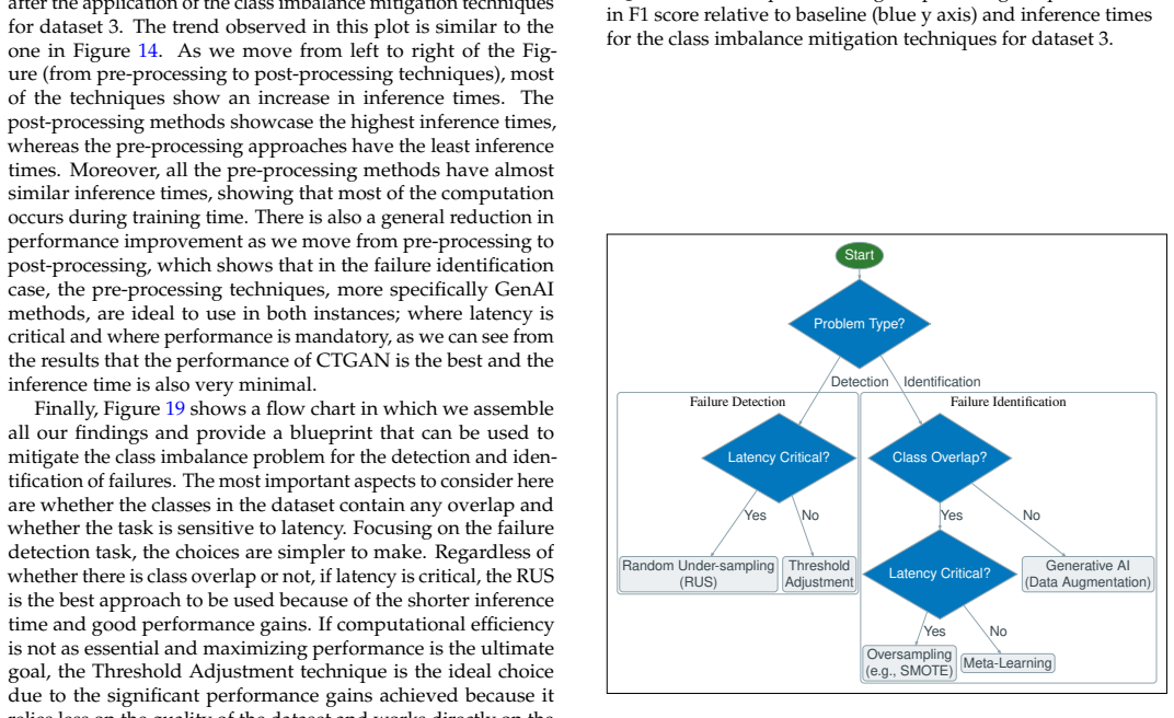
The central organizing device is the pre/in/post-processing taxonomy, with the Fisher Discriminant Ratio (FDR) used as a scalar measure of class overlap that predicts when generative methods will succeed. The load-bearing algorithmic object for the detection result is Algorithm 1, a threshold search that scans candidate probability thresholds and selects the one maximizing F1 on labeled predictions. For the identification result, the load-bearing objects are CTGAN and CVAE, conditional generative models that synthesize minority-class tabular samples. The paper's practical output is a decision flowchart combining problem type, class overlap, and latency.
What would settle it
Run the same twenty methods with a strict three-way split: tune the threshold, costs, and reweighting scale on a validation fold, then report F1 on a held-out test fold. If Threshold Adjustment's margin over Random Under-Sampling and the baseline shrinks below 15.3% or reverses, the claim that post-processing is best for detection fails.
Extended reading notes
Core claim
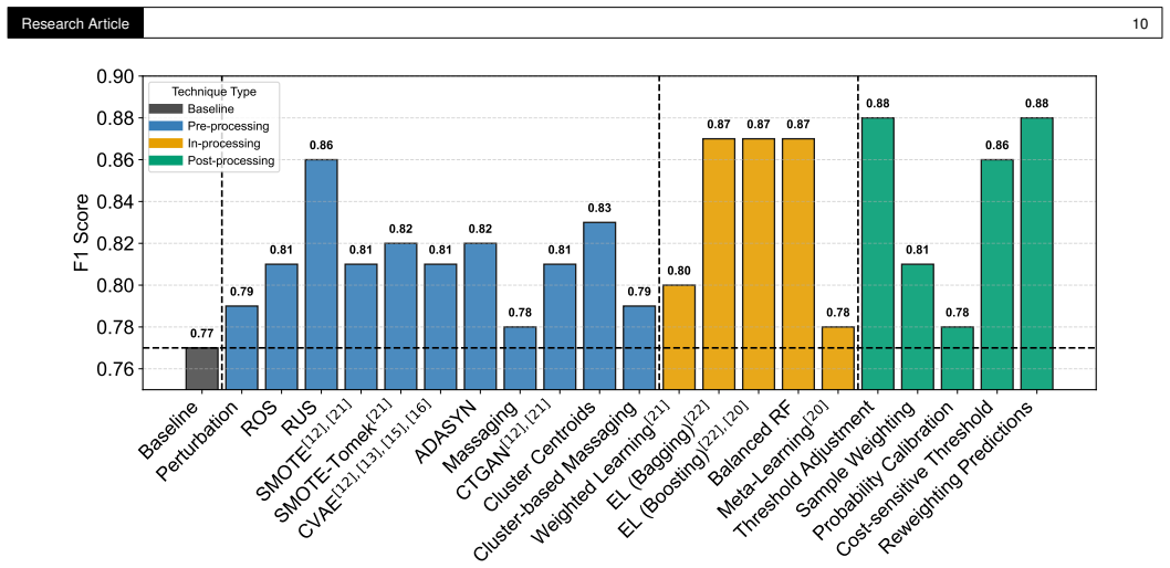
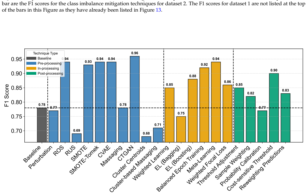
Across experimental optical-network datasets with different degrees of class overlap, the paper claims that no single imbalance-mitigation technique dominates. For failure detection, post-processing methods—particularly Threshold Adjustment, which searches the probability threshold that maximizes F1—outperform all pre- and in-processing alternatives, raising F1 by up to 15.3% over baseline with the lowest variance across runs. For failure identification, generative AI methods, especially CTGAN, provide the largest improvement, up to 24.2%, when classes are well separated. The paper attributes this to the Fisher Discriminant Ratio: when classes overlap heavily, generative models produce poor
Load-bearing premise
The headline F1 gains assume the optimal threshold, cost values, and reweighting scale are chosen on data separate from the data used to report the score; if the same labeled examples were used for both tuning and scoring, the gains would look better than they truly are.
Editorial extensions
If this is right
- For binary failure detection, operators with an already-trained model can get the largest F1 gain by re-tuning the decision threshold on the model's output probabilities, without retraining or resampling.
- For multi-class failure identification with well-separated classes, synthetic minority-class data from CTGAN provides the biggest gain, but post-processing methods require careful per-class tuning and give smaller improvements.
- When inference latency is critical, Random Under-Sampling is the recommended choice for detection despite not being the top performer in F1.
- Class overlap, measured by FDR, is a useful predictor of method family: generative AI fails in low-FDR (overlapping) datasets and excels in high-FDR (separable) datasets.
- The choice of mitigation strategy reduces to a small set of questions—detection vs identification, overlap vs separation, latency-critical vs not—rather than a single universally best method.
Reading between the lines
- An implication not drawn in the paper: for networks that already have deployed failure detectors, threshold adjustment may deliver most of the benefit of data rebalancing at near-zero operational cost, since it touches only the prediction layer.
- The paper's FDR-based explanation suggests a cheap, testable diagnostic: compute the average Fisher Discriminant Ratio on monitoring features first, then select a method family; this could be validated on other tasks such as failure localization.
- Because the reported F1 numbers are computed after tuning threshold, cost values, and reweighting scale on the same labeled data used for evaluation, a strict train/validation/test split could change the size of the 15.3% and 24.2% gains. This is an open question, not a claim the paper makes.
- The overlap-dependent ranking likely extends beyond optical networks to other imbalanced tabular classification problems with continuous features, though the paper only argues for the optical-network setting.
Editorial analysis
A structured set of objections, weighed in public.
Referee Report
Summary. The paper presents a comparative study of pre-, in-, and post-processing class-imbalance mitigation techniques for failure detection and failure identification in optical networks, using three experimental datasets with varying class overlap. The central claims are that post-processing Threshold Adjustment gives the largest F1 improvement (up to 15.3%) for binary failure detection, Generative AI methods (especially CTGAN) give the largest gains (up to 24.2%) for multi-class failure identification, and that method choice should depend on class overlap and latency constraints. The evaluation averages results over 100 runs and uses FDR and PCA to characterize dataset separability.
Significance. If the reported improvements and rankings are unbiased, the paper would be a useful practical benchmark for an under-explored direction, with broad method coverage and validation on experimental testbed data. The use of 100-run averaging and VMR for selected methods is a positive feature. However, the evaluation protocol as described permits post-processing parameters to be tuned on the same labels whose F1 is then reported, which directly affects the headline improvements and the decision blueprint. The contribution is therefore conditional on a corrected evaluation protocol.
major comments (3)
- [Section 3 / 4.A, Algorithm 1, Eq. (5), Section C.3] The headline F1 improvements may be optimistically biased because the paper does not describe a held-out validation split. Algorithm 1 takes 'Predicted probabilities ŷ, True labels y' and searches τ to maximize F1 on those labels; Section C.3 says the Reweighting scaling factor 'can be tuned to maximize the optimization metric'; and Eq. (5) requires misclassification costs CFP/CFN that must be set. If these parameters are selected using the same test labels whose F1 is then reported, the 15.3% Threshold Adjustment gain (Fig. 13) and the 16.4% Cost-sensitive Threshold gain (Fig. 17) are inflated. This is load-bearing because the rankings and the Fig. 19 blueprint rest on these numbers. Please add an explicit train/validation/test split, select all tuning parameters on the validation set, and report test F1 with confidence intervals.
- [Section 4.A/4.B, Figs. 13, 16, 17] The paper makes comparative claims about methods whose F1 scores differ by only a few percentage points, but it reports only averages over 100 runs. No standard deviations, error bars, or significance tests are provided; VMR is reported for only three methods in Fig. 15. Without variance estimates, the cross-method ranking and statements such as 'post-processing has limited impact' in multi-class settings are not statistically supported. Please report per-method variability and use paired tests or confidence intervals for the key comparisons.
- [Section 4.A, Figs. 14, 18] The inference-time comparisons are central to the latency-critical recommendations (RUS fastest, Threshold Adjustment slower, CTGAN minimal inference time), but the measurement protocol is absent. No hardware details, number of timing repetitions, units, or axis labels are given in Figs. 14 and 18, and no variance or confidence intervals are reported for timings. Add a concrete timing protocol so the latency claims can be assessed.
minor comments (4)
- [Section 2.C, Algorithm 2] The statement at the end of Section 2.C that post-processing methods 'do not change the learned decision function' is contradicted by Algorithm 2 (Sample Weighting), which retrains the model on reweighted training data. Please either reclassify this method or revise the statement.
- [Figures 13, 14, 17, 18] Several figures contain garbled placeholder tokens (e.g., '/uni00000025/...') and missing axis labels/units, making the quantitative results difficult to verify. Please regenerate the figures with readable labels and value annotations.
- [Section 2.A.5, Eq. (1)] The Perturbation formula uses rand() without specifying the random-number generation policy or seed. Since results are averaged over 100 runs, please state whether the same seed/process was used across methods.
- [Section 3.A, Section 3.B] The choice of model differs between failure detection (Random Forest) and failure identification (Neural Network), and the RF uses default scikit-learn parameters while the NN uses parameters from [13]. Please justify this asymmetry explicitly, since it may affect cross-task comparisons.
Circularity Check
Threshold Adjustment's headline 15.3% F1 gain is the optimized F1 over the same labels used to select the threshold; absent a described validation split, the detection ranking is partially circular.
-
fitted input called prediction
[Section 2.C.1 (Algorithm 1), Section 2.C.2 Eq. (5), Section 2.C.3, Section 4.A (Fig. 13)]
"Algorithm 1. Threshold Adjustment to Maximize F1-Score: Require: Predicted probabilities ˆy, True labels y ... Compute F1-score: F1 ← F1_score(y, ˆypred) ... select the one that maximizes the F1-score. ... Threshold Adjustment and Reweighting Predictions provide the most notable improvement, increasing the F1 score by up to 15.3% over the baseline."
Algorithm 1 chooses τ to maximize F1 computed on the true labels y supplied as input. The paper never describes a held-out validation set; Section 4.A then reports the resulting F1 as the improvement 'up to 15.3%.' As written, the reported gain is max_τ F1(y, 1(ŷ≥τ)) on the same labels used for selection, so the headline detection gain is the optimized objective rather than an unbiased prediction. The same pattern appears in Eq. (5), where costs are chosen to 'achieve the optimal F1-score,' and in Section C.3, where the scaling factor is 'tuned to maximize the optimization metric.' This makes the post-processing-over-pre/in-processing ranking for detection partially forced by construction.
full rationale
The paper is a broad empirical comparison, not a derivation, and most of its content is self-contained: the experimental datasets, the RF/NN baselines, and standard implementations of SMOTE, CTGAN, ensemble learning, etc., are described or cited to independent sources. The self-citations to Refs. [13] and [52] provide experimental data and baseline hyperparameters; they are not used to forbid alternatives or to import a uniqueness result, so they do not constitute circularity. The one substantial circularity concern is the threshold/cost/reweighting tuning protocol: Algorithm 1 explicitly optimizes F1 on the supplied true labels, and the paper never states that these labels are a validation set distinct from the test set whose F1 is reported. If they are the same labels, the reported 15.3% detection gain is the maximum F1 over thresholds on that label set, so the claim that post-processing 'provides the most expressive improvement' is partially an artifact of test-set fitting rather than an unbiased estimate. This affects the detection ranking but not the identification claim (CTGAN +24.2%), which is a pre-processing augmentation result with no equivalent test-time fit. Hence partial circularity, score 6.
Assumptions & free parameters
free parameters (5)
- F1-optimal threshold tau* =
not reported (scanned in 0-1)
- Reweighting scaling factor =
not reported
- Misclassification costs CFP/CFN =
not reported
- Focal loss parameters gamma, alpha =
not reported
- SMOTE k-nearest neighbors =
not reported
assumptions (3)
- domain assumption Average FDR computed from Eq. (6) is a valid scalar proxy for class overlap/separability in the feature space.
- domain assumption The experimental datasets from [52] and [13] are representative of real optical-network failure data, and end-to-end BER/OSNR monitoring captures the relevant failure signal.
- domain assumption Default scikit-learn RF parameters and the NN architecture from [13] constitute adequate baselines.
Cite this review
Pith. "Pith review of From Data to Decision: A Multi-Stage Framework for Class Imbalance Mitigation in Optical Network Failure Analysis." pith.science (2026). https://pith.science/paper/NL7RGM2H
@misc{pith2026250900057,
  author       = {Pith},
  title        = {Pith review of: From Data to Decision: A Multi-Stage Framework for Class Imbalance Mitigation in Optical Network Failure Analysis},
  year         = {2026},
  howpublished = {\url{https://pith.science/paper/NL7RGM2H}},
  note         = {Machine review of arXiv:2509.00057}
}
read the original abstract
Machine learning-based failure management in optical networks has gained significant attention in recent years. However, severe class imbalance, where normal instances vastly outnumber failure cases, remains a considerable challenge. While pre- and in-processing techniques have been widely studied, post-processing methods are largely unexplored. In this work, we present a direct comparison of pre-, in-, and post-processing approaches for class imbalance mitigation in failure detection and identification using an experimental dataset. For failure detection, post-processing methods-particularly Threshold Adjustment-achieve the highest F1 score improvement (up to 15.3%), while Random Under-Sampling provides the fastest inference. In failure identification, GenAI methods deliver the most substantial performance gains (up to 24.2%), whereas post-processing shows limited impact in multi-class settings. When class overlap is present and latency is critical, over-sampling methods such as the SMOTE are most effective; without latency constraints, Meta-Learning yields the best results. In low-overlap scenarios, Generative AI approaches provide the highest performance with minimal inference time.
Figures


Figures from the paper (15 more)





Reference graph
Works this paper leans on
-
[1]
D. Dass, D. Kilper, L. Barry, and M. Ruffini, “Heterogeneous transmis- sion of analog radio and digital coherent signals over multispan metro and pon for bandwidth-efficient fronthaul in mmwave centralized rans,” J. Opt. Commun. Netw. 17, C136–C143 (2025)
work page 2025
-
[2]
Pca-assisted clustering approaches for soft-failure detection in optical networks,
A. Ribeiro, F . Lobato, M. Silva, A. Sgambelluri, L. Valcarenghi, L. Wosin- ska, and J. Costa, “Pca-assisted clustering approaches for soft-failure detection in optical networks,” J. Opt. Commun. Netw. 17, B50–B60 (2025)
work page 2025
-
[3]
A review of machine learning-based failure management in optical networks,
D. Wang, C. Zhang, W. Chen, H. Y ang, M. Zhang, and A. P . T. Lau, “A review of machine learning-based failure management in optical networks,” Sci. China Inf. Sci. 65, 211302 (2022)
work page 2022
-
[4]
F . Musumeci and M. Tornatore, “Failure management in optical net- works with ML: a tutorial on applications, challenges, and pitfalls,” J. Opt. Commun. Netw. 17, C144–C155 (2025)
work page 2025
-
[5]
Failure management overview in optical networks,
S. Cruzes, “Failure management overview in optical networks,” IEEE Access 12, 169170–169193 (2024)
work page 2024
-
[6]
Y . Wang, C. Zhang, J. Li, Y . Pang, L. Zhang, M. Zhang, and D. Wang, “Alarmgpt: an intelligent alarm analyzer for optical networks using a generative pre-trained transformer,” J. Opt. Commun. Netw.16, 681– 694 (2024)
work page 2024
-
[7]
A tutorial on machine learning for failure management in optical networks,
F . Musumeci, C. Rottondi, G. Corani, S. Shahkarami, F . Cugini, and M. Tornatore, “A tutorial on machine learning for failure management in optical networks,” J. Light. Technol.37, 4125–4139 (2019)
work page 2019
-
[8]
Datasets for qot estimation in SDM networks,
H. Akbari, B. Shariati, J. L. Moreno Morrone, P . Safari, J. K. Fischer, and R. Freund, “Datasets for qot estimation in SDM networks,” J. Opt. Commun. Netw. 17, 514–525 (2025)
work page 2025
Show all 55 references
-
[9]
Open-source data for qot estimation in optical networks from Alibaba,
Z. Zhai, L. Dou, Y . He, A. P . T. Lau, and C. Xie, “Open-source data for qot estimation in optical networks from Alibaba,” J. Opt. Commun. Netw. 16, 1–3 (2023)
2023
-
[10]
Experimental dataset for developing and testing ML models in optical communication systems,
C. Santos, A. Moawad, B. Shariati, R. Emmerich, P . Safari, C. Schubert, and J. K. Fischer, “Experimental dataset for developing and testing ML models in optical communication systems,” J. Opt. Commun. Netw. 16, G1–G10 (2024)
2024
-
[11]
ML-assisted qot estimation: a dataset collection and data visualization for dataset quality evaluation,
G. Bergk, B. Shariati, P . Safari, and J. K. Fischer, “ML-assisted qot estimation: a dataset collection and data visualization for dataset quality evaluation,” J. Opt. Commun. Netw.14, 43–55 (2021)
2021
-
[12]
Addressing data scarcity in ML- based failure-cause identification in optical networks through generative models,
M. Healy, A. Baum, and F . Musumeci, “Addressing data scarcity in ML- based failure-cause identification in optical networks through generative models,” Opt. Fiber Technol.90, 104137 (2025)
2025
-
[13]
Data augmentation to improve performance of neural networks for failure management in optical networks,
L. Z. Khan, J. Pedro, N. Costa, L. De Marinis, A. Napoli, and N. Sambo, “Data augmentation to improve performance of neural networks for failure management in optical networks,” J. Opt. Commun. Netw.15, 57–67 (2022)
2022
-
[14]
A GAN based soft failure detection and identification framework for long- haul coherent optical communication systems,
H. Lun, M. Fu, Y . Zhang, H. Jiang, L. Yi, W. Hu, and Q. Zhuge, “A GAN based soft failure detection and identification framework for long- haul coherent optical communication systems,” J. Light. Technol.41, 2312–2322 (2023)
2023
-
[15]
Data augmentation to reduce computational complexity of neural- network-based soft-failure cause identifier,
L. Z. Khan, P . J. Freire, J. Pedro, N. Costa, A. Napoli, and N. Sambo, “Data augmentation to reduce computational complexity of neural- network-based soft-failure cause identifier,” in 2023 Optical Fiber Com- munications Conference and Exhibition (OFC), (IEEE, 2023), pp. 1–3
2023
-
[16]
The potential of data augmentation for failure management in opti- cal networks,
N. Sambo, L. Z. Khan, J. Pedro, N. Costa, L. De Marinis, and A. Napoli, “The potential of data augmentation for failure management in opti- cal networks,” in Photonic Networks and Devices, (Optica Publishing Group, 2023), pp. NeM3B–1
2023
-
[17]
Monitoring data augmentation of spectral information using VAE and GAN for soft-failure identification,
L. E. Kruse, S. Kühl, A. Dochhan, and S. Pachnicke, “Monitoring data augmentation of spectral information using VAE and GAN for soft-failure identification,” in Optical Fiber Communication Conference, (Optica Publishing Group, 2024), pp. M3I–4
2024
-
[18]
Failure data augmentation for optical network equipment using time-series gen- erative adversarial networks,
C. Xing, C. Zhang, B. Y e, D. Wang, Y . Jia, J. Li, and M. Zhang, “Failure data augmentation for optical network equipment using time-series gen- erative adversarial networks,” in 2023 Optical Fiber Communications Conference and Exhibition (OFC), (IEEE, 2023), pp. 1–3
2023
-
[19]
Application of ML al- gorithms for prediction of the QoT in optical networks with imbal- anced and incomplete data,
P . Cichosz, S. Kozdrowski, and S. Sujecki, “Application of ML al- gorithms for prediction of the QoT in optical networks with imbal- anced and incomplete data,” in 2021 International Conference on Software, T elecommunications and Computer Networks (SoftCOM), (IEEE, 2021), pp. 1–6
2021
-
[20]
A Stacking En- semble ML-Based Failure Prediction Model for Optical Networks with Imbalanced Data,
Z. Sun, C. Zhang, M. Zhang, F . Y ang, and D. Wang, “A Stacking En- semble ML-Based Failure Prediction Model for Optical Networks with Imbalanced Data,” in 2023 Asia Communications and Photonics Con- ference/2023 International Photonics and Optoelectronics Meetings Research Ar...
2023
-
[21]
Model and data-centric machine learning algorithms to address data scarcity for failure identification,
L. Z. Khan, J. Pedro, N. Costa, A. Sgambelluri, A. Napoli, and N. Sambo, “Model and data-centric machine learning algorithms to address data scarcity for failure identification,” J. Opt. Commun. Netw. 16, 369–381 (2024)
2024
-
[22]
Shap-assisted ee-lightgbm model for explainable fault diagnosis in practical optical networks,
C. Zhang, Y . Chen, M. Zhang, Z. Liu, and D. Wang, “Shap-assisted ee-lightgbm model for explainable fault diagnosis in practical optical networks,” J. Opt. Commun. Netw. 17, 81–94 (2025)
2025
-
[23]
Survey on machine learning biases and mitigation techniques,
S. Siddique, M. A. Haque, R. George, K. D. Gupta, D. Gupta, and M. J. H. Faruk, “Survey on machine learning biases and mitigation techniques,” Digital. 4, 1–68 (2023)
2023
-
[24]
Bias mitiga- tion for machine learning classifiers: A comprehensive survey,
M. Hort, Z. Chen, J. M. Zhang, M. Harman, and F . Sarro, “Bias mitiga- tion for machine learning classifiers: A comprehensive survey,” ACM J. on Responsible Comput. 1, 1–52 (2024)
2024
-
[25]
Rwo-sampling: A random walk over-sampling approach to imbalanced data classification,
H. Zhang and M. Li, “Rwo-sampling: A random walk over-sampling approach to imbalanced data classification,” Inf. Fusion 20, 99–116 (2014)
2014
-
[26]
Smote: synthetic minority over-sampling technique,
N. V. Chawla, K. W. Bowyer, L. O. Hall, and W. P . Kegelmeyer, “Smote: synthetic minority over-sampling technique,” J. artificial intelligence research 16, 321–357 (2002)
2002
-
[27]
K-nearest neighbour classifiers-a tutorial,
P . Cunningham and S. J. Delany, “K-nearest neighbour classifiers-a tutorial,” ACM computing surveys (CSUR) 54, 1–25 (2021)
2021
-
[28]
Adasyn: Adaptive synthetic sampling approach for imbalanced learning,
H. He, Y . Bai, E. A. Garcia, and S. Li, “Adasyn: Adaptive synthetic sampling approach for imbalanced learning,” in 2008 IEEE interna- tional joint conference on neural networks (IEEE world congress on computational intelligence), (Ieee, 2008), pp. 1322–1328
2008
-
[29]
The effects of random undersampling with simulated class imbalance for big data,
T. Hasanin and T. Khoshgoftaar, “The effects of random undersampling with simulated class imbalance for big data,” in2018 IEEE international conference on information reuse and integration (IRI), (IEEE, 2018), pp. 70–79
2018
-
[30]
Clustering-based undersampling in class-imbalanced data,
W.-C. Lin, C.-F . Tsai, Y .-H. Hu, and J.-S. Jhang, “Clustering-based undersampling in class-imbalanced data,” Inf. Sci. 409, 17–26 (2017)
2017
-
[31]
Unsupervised k-means clustering algo- rithm,
K. P . Sinaga and M.-S. Y ang, “Unsupervised k-means clustering algo- rithm,” IEEE Access 8, 80716–80727 (2020)
2020
-
[32]
A study of the behavior of several methods for balancing machine learning training data,
G. E. Batista, R. C. Prati, and M. C. Monard, “A study of the behavior of several methods for balancing machine learning training data,” ACM SIGKDD Explor. Newsl. 6, 20–29 (2004)
2004
-
[33]
Two modifications of CNN,
I. Tomek, “Two modifications of CNN,” IEEE Transactions on Syst. Man Cybern. 11, 769–772 (1976)
1976
-
[34]
Generative adversarial nets,
I. J. Goodfellow, J. Pouget-Abadie, M. Mirza, B. Xu, D. Warde-Farley, S. Ozair, A. Courville, and Y . Bengio, “Generative adversarial nets,” Adv. Neural Inf. Process. Syst. 27 (2014)
2014
-
[35]
Generative adversarial networks (GANs) chal- lenges, solutions, and future directions,
D. Saxena and J. Cao, “Generative adversarial networks (GANs) chal- lenges, solutions, and future directions,” ACM Comput. Surv. (CSUR) 54, 1–42 (2021)
2021
-
[36]
Modeling tabular data using conditional GAN,
L. Xu, M. Skoularidou, A. Cuesta-Infante, and K. Veeramacha- neni, “Modeling tabular data using conditional GAN,” arXiv preprint arXiv:1907.00503 (2019)
1907 arXiv
-
[37]
Wasserstein generative ad- versarial networks,
M. Arjovsky, S. Chintala, and L. Bottou, “Wasserstein generative ad- versarial networks,” in International conference on machine learning, (PMLR, 2017), pp. 214–223
2017
-
[38]
Auto-encoding variational bayes,
D. P . Kingma and M. Welling, “Auto-encoding variational bayes,” (2013)
2013
-
[39]
Tutorial on variational autoencoders,
C. Doersch, “Tutorial on variational autoencoders,” arXiv preprint arXiv:1606.05908 (2016)
2016 arXiv
-
[40]
Class weighting technique to deal with imbalanced class problem in machine learning: Methodological re- search,
B. Bakirarar and A. H. Elhan, “Class weighting technique to deal with imbalanced class problem in machine learning: Methodological re- search,” Türkiye Klinikleri Biyoistatistik 15, 19–29 (2023)
2023
-
[41]
Focal loss for dense object detection,
T.-Y . Lin, P . Goyal, R. Girshick, K. He, and P . Dollár, “Focal loss for dense object detection,” in Proceedings of the IEEE international con- ference on computer vision, (2017), pp. 2980–2988
2017
-
[42]
Ensemble learning: A survey,
O. Sagi and L. Rokach, “Ensemble learning: A survey,” Wiley interdisci- plinary reviews: data mining knowledge discovery 8, e1249 (2018)
2018
-
[43]
Exploratory undersampling for class- imbalance learning,
X.-Y . Liu, J. Wu, and Z.-H. Zhou, “Exploratory undersampling for class- imbalance learning,” IEEE Transactions on Syst. Man, Cybern. Part B (Cybernetics) 39, 539–550 (2008)
2008
-
[44]
C. Chen, A. Liaw, L. Breiman et al. , Using random forest to learn imbalanced data. Technical report (University of California, Berkeley, 2004)
2004
-
[45]
Advances and challenges in meta-learning: A technical review,
A. Vettoruzzo, M.-R. Bouguelia, J. Vanschoren, T. Rögnvaldsson, and K. Santosh, “Advances and challenges in meta-learning: A technical review,” IEEE Transactions on Pattern Analysis Mach. Intell.46, 4763– 4779 (2024)
2024
-
[46]
Finding the best classification threshold in imbalanced classification,
Q. Zou, S. Xie, Z. Lin, M. Wu, and Y . Ju, “Finding the best classification threshold in imbalanced classification,” Big Data Res. 5, 2–8 (2016)
2016
-
[47]
Cost-sensitive learning for imbalanced medical data: a review,
I. Araf, A. Idri, and I. Chairi, “Cost-sensitive learning for imbalanced medical data: a review,” Artif. Intell. Rev. 57, 80 (2024)
2024
-
[48]
Calibration of probabil- ities: The state of the art,
S. Lichtenstein, B. Fischhoff, and L. D. Phillips, “Calibration of probabil- ities: The state of the art,” in Decision Making and Change in Human Affairs: Proceedings of the Fifth Research Conference on Subjective Probability , Utility , and Decision Making, Darmstadt, 1–4 Sep...
1975
-
[49]
Probabilistic outputs for support vector machines and compar- isons to regularized likelihood methods,
J. Platt, “Probabilistic outputs for support vector machines and compar- isons to regularized likelihood methods,” Adv. Large Margin Classif.10, 61–74 (1999)
1999
-
[50]
Transforming classifier scores into accurate multiclass probability estimates,
B. Zadrozny and C. Elkan, “Transforming classifier scores into accurate multiclass probability estimates,” in Proceedings of the eighth ACM SIGKDD international conference on Knowledge discovery and data mining, (2002), pp. 694–699
2002
-
[51]
Predicting good probabilities with supervised learning,
A. Niculescu-Mizil and R. Caruana, “Predicting good probabilities with supervised learning,” in Proceedings of the 22nd international confer- ence on Machine learning, (2005), pp. 625–632
2005
-
[52]
Learning long-and short-term temporal patterns for ML-driven fault management in optical communication networks,
M. F . Silva, A. Pacini, A. Sgambelluri, and L. Valcarenghi, “Learning long-and short-term temporal patterns for ML-driven fault management in optical communication networks,” IEEE Transactions on Netw. Serv. Manag. 19, 2195–2206 (2022)
2022
-
[53]
Principal component analysis: a review and recent developments,
I. T. Jolliffe and J. Cadima, “Principal component analysis: a review and recent developments,” Philos. Transactions Royal Soc. A: Math. Phys. Eng. Sci. 374, 20150202 (2016)
2016
-
[54]
Adaptive feature selection through fisher discriminant ratio,
K. Kalinkov, T. Ganchev, and V. Markova, “Adaptive feature selection through fisher discriminant ratio,” in 2019 International Conference on Biomedical Innovations and Applications (BIA), (IEEE, 2019), pp. 1–4
2019
-
[55]
Scikit-learn: Machine learning in python,
F . Pedregosa, G. Varoquaux, A. Gramfort, V. Michel, B. Thirion, O. Grisel, M. Blondel, P . Prettenhofer, R. Weiss, V. Dubourg et al. , “Scikit-learn: Machine learning in python,” J. Mach. Learn. Res. 12, 2825–2830 (2011)
2011
Reviewed August 5, 2026 · model on record in the stance chip above.
Discussion (0). Sign in to comment.