REVIEW 2 major objections 3 minor 21 references
Discrete efficiency choices in deep learning become continuous objectives that train end-to-end.
Reviewed by Pith at T0; open to challenge. T0 means a machine referee read the full paper against a public rubric. the ladder, T0–T4 →
A thesis that synthesizes the author's published work on continuous approximations to discrete deep learning problems, with experiments showing efficiency gains, but offering little new beyond the author's prior papers.
T0 review reviewed 2026-08-05 challenge →
load-bearing objection A transparent, well-run thesis that repackages the author's own strong prior work; the 'principled' quantization claim has a load-bearing assumption that is likely false under the paper's own bit map. the 2 major comments →
Principled Approximation Methods for Efficient and Scalable Deep Learning
The pith
A machine-rendered reading of the paper's core claim, the machinery that carries it, and where it could break.
The reading
Core claim
The central claim is that computationally intractable discrete optimization problems in deep learning can be replaced by principled continuous approximations that remain faithful to the original problem as a parameter approaches a limit. For sparsification, the binary keep/drop mask becomes σ(βs), and annealing β upward drives weights smoothly out of the network, recovering ℓ0 regularization in the limit. For quantization, precision assignment is re-framed as an infinite-constraint problem and then approximated stochastically: each weight learns a perturbation scale that captures how much noise it tolerates, and that scale is converted into a bit precision. For architecture search, each laye
What carries the argument
The unifying mechanism is the continuous relaxation with an annealing or scale parameter. In Continuous Sparsification it is the sigmoidal mask σ(βs) on each weight, with β annealed so the smooth objective converges to the ℓ0-penalized discrete problem. In SMOL it is the perturbation proxy: each precision variable s defines a noise magnitude σ(s), and the loss is computed on w+σ(s)⊙ε, so gradients through the noise magnitude reveal how much precision each weight can give up. In the architecture search chapter it is the template mixing coefficient α, which expresses each layer's effective weight as a linear combination of shared templates and yields a layer-similarity matrix that the method f
Load-bearing premise
The quantization results rest on the assumption that adding precision to a weight never turns an acceptable quantized model into an unacceptable one; if that monotonicity fails, the reformulated objective is not equivalent to the original mixed-precision problem.
What would settle it
Run SMOL's precision training on a small network, then take the assigned per-weight precisions and measure the loss for strictly higher-precision versions of the same weights. If increasing precision ever raises the loss, or if lowering a judged-infeasible precision stays within the δ tolerance, the monotonic-satisfiability and density assumptions that underwrite the method are violated.
If this is right
- Compression need not be a post-hoc step: mask and precision variables receive gradient updates alongside weights, so the compression scheme is learned while the model trains.
- Per-weight and per-layer precision allocation can be optimized by gradient descent, producing non-uniform bit assignments that reduce total bits while preserving accuracy.
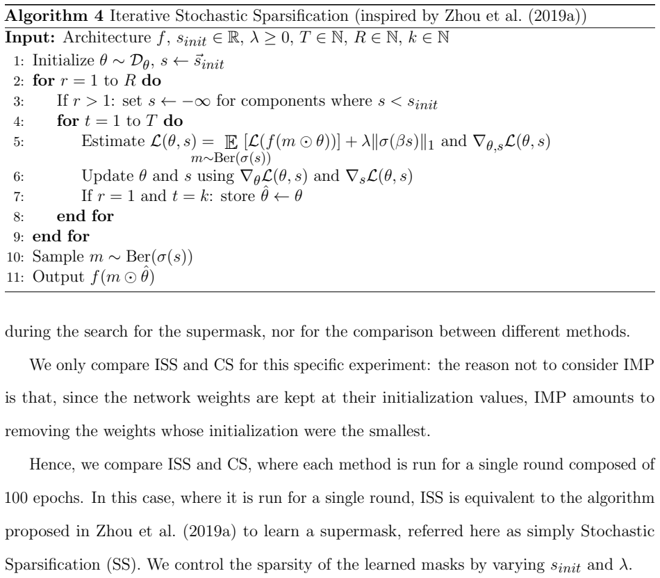
- Ticket search—finding sparse subnetworks that train from scratch—becomes cheaper than iterative magnitude pruning when runs are parallelized, and the discovered tickets can match or exceed the dense model's accuracy.
- Architecture search over a topological space can discover recurrent/looped structures from feedforward CNN seeds, and the layer-similarity matrix provides a concrete recipe for folding them into smaller equivalent networks.
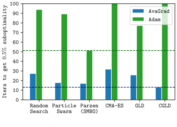
- The adaptive optimizer's design makes learning rate and adaptability near-separable, so hyperparameter optimization reaches a target accuracy in fewer trials than Adam.
Where Pith is reading between the lines
- The perturbation-limit principle is a general sensitivity measure: it could be used to set tolerances for other discretizations—activation quantization, block-wise formats, or reduced-precision training—without repeating the full derivation.
- The monotonic satisfiability assumption behind SMOL suggests its precision assignments are conservative: in regimes where extra precision can hurt, an over-precision penalty or a validation-based correction might improve bit savings.
- The layer-similarity folding analysis could serve as a diagnostic for implicit recurrence in any trained network, independent of whether the network was produced by this search procedure.
- A joint objective that anneals both the sparsification mask and the quantization scale would combine two compression axes into a single continuous relaxation; the ingredients for it appear in different chapters of the thesis.
Editorial analysis
A structured set of objections, weighed in public.
Referee Report
Summary. This PhD thesis proposes and evaluates continuous, differentiable approximations to three discrete optimization problems arising in deep learning efficiency, plus a modified adaptive optimizer. Chapter 3 relaxes neural architecture search over a topological search space via soft parameter sharing; Chapter 4 relaxes ℓ0 sparsification using an annealed sigmoid mask, yielding Continuous Sparsification (CS); Chapter 5 derives a perturbation-based method, SMOL, for mixed-precision quantization; Chapter 6 analyzes adaptive methods and proposes AvaGrad. The experimental sections are extensive, covering CIFAR, ImageNet, IWSLT, GANs, and various architectures, and the thesis claims substantial improvements in parameter efficiency, sparsity, precision allocation, and hyperparameter tuning cost.
Significance. If the central claims hold, the thesis is practically significant: CS finds extremely sparse subnetworks with less computation than iterative magnitude pruning; SMOL demonstrates fine-grained precision assignment that can outperform uniform-precision baselines; and AvaGrad shows competitive accuracy with reduced hyperparameter sensitivity. The thesis also contains full proofs for the optimizer convergence results in Chapter 6 and carefully documents ablations and hyperparameter analyses. However, the 'principled approximation' framing is only partially established. For sparsification, the method optimizes a lower bound without a no-gap proof; for quantization, the equivalence with the original mixed-precision problem relies on an unverified monotonicity assumption that is, in fact, false under the paper's own bit-value map. These are load-bearing gaps for the stated theoretical claims, though the empirical methods remain interesting and potentially useful.
major comments (2)
- [§5.2.2, Eq. (5.12)]
- [§4.2.3, Eq. (4.14)]
minor comments (3)
- [§5.2.1]
- [Chapter 6, Tables 6.1 and 6.2]
- [Throughout]
Circularity Check
No significant circularity: the thesis compiles the author's prior peer-reviewed work with self-contained formal derivations and new experiments; no central claim reduces to its own inputs by construction.
full rationale
The thesis is a compilation of four previously published research thrusts (Savarese and Maire 2019; Savarese et al. 2020, 2021, 2022). The self-references are provenance statements, not load-bearing justifications: each chapter re-derives its formal problem, states the discrete objective, introduces a continuous relaxation, and then reports experimental measurements. The approximations are not defined in terms of the target outcomes. For example, Continuous Sparsification instantiates a sigmoid homotopy from a stated ℓ0 objective and explicitly acknowledges the min/limit swap gap (Section 4.2.3, Eq. 4.14); SMOL defines precision via a perturbation proxy and an explicit monotonicity assumption (Eq. 5.12). These are stated assumptions and potential correctness risks, but they are not circular: the re-framed problems are not equivalent to the conclusions by construction, and the paper does not present tuned hyperparameters as predictions. No uniqueness theorem is imported from the authors' prior work, and no benchmark is fitted and then claimed as a forecast. The quantization chapter's reliance on Eq. 5.12 is an unproven and possibly false assumption (the skeptic's counterexample illustrates a robustness issue), but a false or untested assumption is a correctness concern, not circularity. Overall, the derivation chain is self-contained and empirically anchored; the modest self-citation pattern does not constitute circularity.
Axiom & Free-Parameter Ledger
free parameters (5)
- sparsity regularization strength lambda =
10^-8
- annealing temperature beta_final =
200
- mask initialization s_init =
ranges -0.3 to 0.3
- precision regularization lambda =
10^-6, 7e-7, 5e-7, etc.
- initial precision p_init =
8
axioms (4)
- domain assumption Swapping the order of minimization and limit in the sparsification approximation (Section 4.2.3) yields a valid lower bound; requires Gamma-convergence and equi-coercivity of L_beta to ensure no gap in the limit.
- domain assumption Satisfiability is monotone in precision: if (theta,p) is satisfiable then (theta,p') is satisfiable for any p' >= p (Equation 5.12, Section 5.2.2).
- standard math The bit-value map v_j = 2^{1-j} (fixed-point binary) and reparameterization s = sigma^{-1}(2^{1-p}) restrict the method to uniform fixed-point quantization.
- standard math L of f is continuous for the limit-swap justification (Definition 4.4).
Cite this review
Pith. "Pith review of Principled Approximation Methods for Efficient and Scalable Deep Learning." pith.science (2026). https://pith.science/paper/TYS274IM
@misc{pith2026250900174,
  author       = {Pith},
  title        = {Pith review of: Principled Approximation Methods for Efficient and Scalable Deep Learning},
  year         = {2026},
  howpublished = {\url{https://pith.science/paper/TYS274IM}},
  note         = {Machine review of arXiv:2509.00174}
}
read the original abstract
Recent progress in deep learning has been driven by increasingly larger models. However, their computational and energy demands have grown proportionally, creating significant barriers to their deployment and to a wider adoption of deep learning technologies. This thesis investigates principled approximation methods for improving the efficiency of deep learning systems, with a particular focus on settings that involve discrete constraints and non-differentiability. We study three main approaches toward improved efficiency: architecture design, model compression, and optimization. For model compression, we propose novel approximations for pruning and quantization that frame the underlying discrete problem as continuous and differentiable, enabling gradient-based training of compression schemes alongside the model's parameters. These approximations allow for fine-grained sparsity and precision configurations, leading to highly compact models without significant fine-tuning. In the context of architecture design, we design an algorithm for neural architecture search that leverages parameter sharing across layers to efficiently explore implicitly recurrent architectures. Finally, we study adaptive optimization, revisiting theoretical properties of widely used methods and proposing an adaptive optimizer that allows for quick hyperparameter tuning. Our contributions center on tackling computationally hard problems via scalable and principled approximations. Experimental results on image classification, language modeling, and generative modeling tasks show that the proposed methods provide significant improvements in terms of training and inference efficiency while maintaining, or even improving, the model's performance.
Figures








Reference graph
Works this paper leans on
-
[1]
Yoshua Bengio, Nicholas L´ eonard, and Aaron Courville. Estimating or propagating gradients through stochastic neurons for conditional computation.arXiv:1308.3432, 2013a. Yoshua Bengio, Nicholas L´ eonard, and Aaron Courville. Estimating or propagating gradients through stochastic neurons for conditional computation.arXiv:1308.3432, 2013b. Alexandre Boulc...
-
[4]
Jonathan Frankle, Gintare Karolina Dziugaite, Daniel M. Roy, and Michael Carbin. Stabilizing the lottery ticket hypothesis.arXiv:1903.01611,
Pith/arXiv arXiv 1903
-
[5]
Neural Turing Machines.arXiv:1410.5401,
Alex Graves, Greg Wayne, and Ivo Danihelka. Neural Turing Machines.arXiv:1410.5401,
-
[11]
An Analysis of Neural Language Modeling at Multiple Scales.arXiv:1803.08240,
Stephen Merity, Nitish Shirish Keskar, and Richard Socher. An Analysis of Neural Language Modeling at Multiple Scales.arXiv:1803.08240,
-
[13]
Regularized evolution for image classifier architecture search.arXiv:1802.01548,
Esteban Real, Alok Aggarwal, Yanping Huang, and Quoc V Le. Regularized evolution for image classifier architecture search.arXiv:1802.01548,
-
[16]
Training Sparse Neural Networks
Suraj Srinivas, Akshayvarun Subramanya, and R. Venkatesh Babu. Training sparse neural networks.arXiv:1611.06694,
work page internal anchor Pith review Pith/arXiv arXiv
-
[17]
ACDC: Weight Sharing in Atom-Coefficient Decomposed Convolution
Ze Wang, Xiuyuan Cheng, Guillermo Sapiro, and Qiang Qiu. Acdc: Weight sharing in atom-coefficient decomposed convolution.arXiv preprint arXiv:2009.02386,
work page internal anchor Pith review Pith/arXiv arXiv 2009
-
[18]
Mixed precision quantization of ConvNets via differentiable neural architecture search
Bichen Wu, Yanghan Wang, Peizhao Zhang, Yuandong Tian, Peter Vajda, and Kurt Keutzer. Mixed precision quantization of ConvNets via differentiable neural architecture search. arXiv:1812.00090,
-
[21]
Deconstructing lottery tickets: Zeros, signs, and the supermask.NeurIPS, 2019a
Hattie Zhou, Janice Lan, Rosanne Liu, and Jason Yosinski. Deconstructing lottery tickets: Zeros, signs, and the supermask.NeurIPS, 2019a. Shuchang Zhou, Zekun Ni, Xinyu Zhou, He Wen, Yuxin Wu, and Yuheng Zou. DoReFa- Net: Training low bitwidth convolutional neural networks with low bitwidth gradients. arXiv:1606.06160,
-
[22]
To prune, or not to prune: exploring the efficacy of pruning for model compression.arXiv:1710.01878,
Michael Zhu and Suyog Gupta. To prune, or not to prune: exploring the efficacy of pruning for model compression.arXiv:1710.01878,
-
[1989]
J. H. Lim and J. C. Ye. Geometric gan.arXiv:1806.06763,
-
[1994]
Sparse transfer learning via winning lottery tickets.arXiv:1905.07785,
Rahul Mehta. Sparse transfer learning via winning lottery tickets.arXiv:1905.07785,
Pith/arXiv arXiv 1905
-
[1997]
MobileNets: Efficient convolutional neural networks for mobile vision applications.arXiv:1704.04861,
Andrew G Howard, Menglong Zhu, Bo Chen, Dmitry Kalenichenko, Weijun Wang, Tobias Weyand, Marco Andreetto, and Hartwig Adam. MobileNets: Efficient convolutional neural networks for mobile vision applications.arXiv:1704.04861,
-
[2010]
Daisuke Miyashita, Edward H. Lee, and Boris Murmann. Convolutional neural networks using logarithmic data representation.arXiv:1603.01025,
-
[2015]
BSQ: Exploring bit-level sparsity for mixed-precision neural network quantization.arXiv:2102.10462,
186 Huanrui Yang, Lin Duan, Yiran Chen, and Hai Li. BSQ: Exploring bit-level sparsity for mixed-precision neural network quantization.arXiv:2102.10462,
-
[2016]
David Ha, Andrew Dai, and Quoc V. Le. Hypernetworks.arXiv:1609.09106,
-
[2017]
Forrest N. Iandola, Matthew W. Moskewicz, Khalid Ashraf, Song Han, William J. Dally, and Kurt Keutzer. SqueezeNet: AlexNet-level accuracy with 50x fewer parameters and <1MB model size.arXiv:1602.07360,
-
[2018]
On the Convergence of AdaBound and its Connection to SGD
Pedro Savarese. On the Convergence of AdaBound and its Connection to SGD. arXiv:1908.04457,
work page internal anchor Pith review Pith/arXiv arXiv 1908
-
[2019]
PACT: Parameterized clipping activation for quantized neural networks.arXiv:1805.06085,
Jungwook Choi, Zhuo Wang, Swagath Venkataramani, Pierce I-Jen Chuang, Vijayalakshmi Srinivasan, and Kailash Gopalakrishnan. PACT: Parameterized clipping activation for quantized neural networks.arXiv:1805.06085,
-
[2020]
Cyrus Zhou, Pedro Savarese, Vaughn Richard, Zack Hassman, Xin Yuan, Michael Maire, Michael DiBrino, and Yanjing Li. SySMOL: Co-designing Algorithms and Hardware for Neural Networks with Heterogeneous Precisions.arXiv:2311.14114,
-
[2023]
184 Gustavo Silva and Paul Rodriguez. Fine-Tuning Adaptive Stochastic Optimizers: De- termining the Optimal Hyperparameter ϵ via Gradient Magnitude Histogram Analysis. arXiv:2311.11532,
work page internal anchor Pith review Pith/arXiv arXiv
This paper was first reviewed by deepseek-v4-flash on August 5, 2026.
discussion (0)
Sign in with ORCID, Apple, or X to comment. Anyone can read and Pith papers without signing in.