REVIEW 3 major objections 5 minor 37 references
Annealed neural samplers train better when the proposal distribution sweeps a continuously varying temperature coordinate, letting samples cross energy barriers where standard annealed Langevin proposals get stuck.
Reviewed by Pith at T0; open to challenge. T0 means a machine referee read the full paper against a public rubric. the ladder, T0–T4 →
CTDS trains neural samplers with a controlled Langevin dynamics over both position and a continuous temperature coordinate, and reports improved sampling on a 40-mode Gaussian mixture.
T0 review reviewed 2026-08-05 challenge →
load-bearing objection A promising NETS extension with a real W2 gain on a single 2D mixture, but the 'extended exploration' story is unmeasured and eq. (19) has a likely typo. the 3 major comments →
Continuously Tempered Diffusion Samplers
The pith
A machine-rendered reading of the paper's core claim, the machinery that carries it, and where it could break.
The reading
Core claim
The proposal distribution that feeds a PINN sampler loss can itself be a tempering scheme. The paper extends the time-indexed annealing path to a density continuum over (t, β), reparameterizes β via a coordinate ξ with plateaus at both endpoints, and runs a controlled underdamped Langevin dynamics on the augmented state (x, ξ). A multi-temperature PINN loss trains the control and a learned free-energy estimate over this continuum; Theorem 3.2, a controlled Jarzynski equality for the tempered dynamics, justifies reweighting samples. On the 40-mode Gaussian mixture, the CTDS sampler reaches W2 = 12.87 ± 0.20 versus 20.11 ± 0.23 for the best baseline, and the reweighted variant gives the best u
What carries the argument
The continuously tempered diffusion sampler (eq. 17): a controlled underdamped Langevin dynamics over the augmented state (x, ξ) with a non-separable Hamiltonian whose kinetic energy weights the position momentum by β(ξ). The reparameterization β(ξ) (eq. 30) maps R onto [β_min, 1] with plateaus at both endpoints, so the temperature marginal spends real time at the target temperature and at the high-temperature end, while a confining potential (eq. 32) keeps ξ in range. Two further pieces carry the argument: the multi-temperature PINN objective (eq. 13), whose unique minimizer over F is the joint free energy (Thm 3.1), and the continuously tempered controlled Jarzynski equality (Thm 3.2), use
Load-bearing premise
The method succeeds only if the temperature coordinate ξ mixes quickly enough that, at every curriculum stage, the proposal spends real time at both the target temperature β=1 and the high-temperature end β_min; if the ξ marginal pools away from β=1 early in training, a failure the authors observe and blame on a poor free-energy estimate, the learned control at β=1, the only temperature used at evaluation, is undertrained.
What would settle it
Record the empirical marginal of ξ from the CTDS proposal at several early curriculum stages on a multimodal target with the free-energy network at initial weights. If the fraction of training samples at β(ξ)=1 is negligible through the first half of training while post-training W2 at β=1 matches the non-tempered baselines, the exploration claim fails. Alternatively, freeze the learned free energy, simulate eq. (17), and check whether any trajectory that reaches the β_min plateau returns to the β=1 plateau within the barrier-crossing time scale; if none do, the mechanism is absent.
If this is right
- Post-training, the CTDS-trained control spreads samples across the modes of the mixture, while controls trained with the ODE-only, overdamped, and underdamped proposals collapse onto fewer modes; the W2 gap (12.87 vs 20.11) is the paper's headline number.
- Because the loss is defined over the whole time–temperature continuum, training is amortized across temperatures: one control network carries the transport for every β, with β=1 recovered at evaluation.
- The Jarzynski-reweighted CTDS reaches the lowest evidence upper bound, indicating the learned density covers the target's mass without leaving regions underweighted.
- The construction only needs energies that scale with β (U^β ∝ βU), so any target whose barriers shrink at higher temperature, the standard tempering assumption, fits the same proposal design, not just Gaussian mixtures.
Where Pith is reading between the lines
- The paper reports that early in training the ξ marginal pools away from β=1 (fig. 2), yet does not measure ξ mixing time or the fraction of training samples at β=1; that fraction is a cheap, direct diagnostic of whether the method's exploration is actually operating at each curriculum stage.
- The non-reweighted CTDS beating the reweighted CTDS on W2 suggests the Jarzynski weights, computed with an early free-energy estimate that is still poor, inject noise; a variance-reduced or progressively annealed weight estimator might combine the best of both rows.
- A natural extension the paper does not explore: run several ξ trajectories with replica-exchange swaps as the proposal instead of one confining-potential trajectory, which could decorrelate the β=1 particles without relying on returns to the plateau.
- The 2D validation leaves high-dimensional behavior open; in higher dimensions the joint free-energy learning over (t, ξ) becomes harder, so whether the exploration gain survives the harder estimation problem is a testable open question.
Editorial analysis
A structured set of objections, weighed in public.
Referee Report
Summary. The paper proposes continuously tempered diffusion samplers (CTDS), an extension of PINN-based annealed neural samplers (NETS) to a time-and-temperature-indexed density continuum. The authors introduce a multi-temperature PINN objective over (x, t, ξ), a continuously tempered underdamped Langevin proposal in the augmented state (x, ξ), and a controlled Jarzynski equality for reweighting the proposal during training. They evaluate CTDS on a 40-mode Gaussian mixture, reporting lower W2 and better ELBO than baseline, overdamped NETS, and underdamped NETS proposals. The paper also provides a proof of the multi-temperature PINN minimizer and a Crooks/Jarzynski derivation in appendices, with code available.
Significance. If the theoretical statements are corrected, the paper makes a useful conceptual contribution: it transfers continuous-tempering ideas from molecular dynamics to amortized neural sampling, and it shows a plausible way to use multi-temperature proposals in PINN-based samplers. The multi-temperature PINN loss and the controlled Jarzynski reweighting are nontrivial extensions of existing single-temperature results, and the public code is a strength. However, the empirical support is limited to one 2D benchmark, and the central mechanistic claim—that improvements are driven by extended exploration—is not directly measured or isolated by an ablation.
major comments (3)
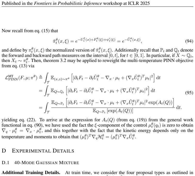
- [Section 3.4, Eq. (19); Appendix C.3, Eqs. (78)/(90)] The work functional is printed with ∂_t log \tilde U^θ_t (and ∂_t log U_t in the appendix). The derivation at Appendix C.3, Eq. (83) yields ∂_t U_t, and the 'log' is not a harmless notation variant: \tilde U is an energy and may be negative or zero. Additionally, Theorem 3.2 defines F_t as ∫ e^{-\tilde U^θ_t} dx dz, which is a partition function Z_t, while the displayed identity E[e^{A_T}] = exp(F_0 − F_T) requires F_t = −log Z_t; as printed, the identity becomes exp(Z_0 − Z_T). Since Eq. (22) relies on this theorem for reweighting, the theorem needs correction before the method is well-defined.
- [Section 4.1, Fig. 2] The abstract claims 'improved sampler performance driven by extended exploration,' but the paper does not measure exploration or the training-time population at β=1. Fig. 2 shows only the ξ marginal at t=1.0 before/after training; it does not report the fraction of training proposals with |ξ|<Δ (i.e., β=1) as the curriculum progresses, nor the mode coverage of the proposal. Because CTDS also adds a temperature input and Fourier features, the W2 gain over NETS could result from the extra capacity or multi-task regularization rather than from the proposed tempering mechanism. Section 3.4 itself notes that with a poor free-energy estimate samples pool away from β=1. Please add an ablation with ξ dynamics frozen at β=1 (or ξ drawn from a fixed distribution) and, if possible, report per-epoch β=1 occupancy and proposal mode coverage.
- [Section 3.1 and Appendix D.1] The formal continuum definition sets π^β_0 = N(0, (1/β)I), i.e., U^β_0 = (β/2)||x||², but the experiments use π0 = N(0, 5I₂). It is ambiguous whether the continuum in the experiments is defined by U^β_0 = β U^1_0 (so the source variance becomes 25/β) or by the canonical U^β_0 = (β/2)||x||² with a different β=1 source. This affects the temperature scaling of the proposal and should be clarified for reproducibility.
minor comments (5)
- [Theorem 3.2 and Eq. (22)] The theorem writes h(x, ξ) but then evaluates h(Q) on a path; Eq. (22) similarly uses P_t as if h were a terminal function. Please state explicitly that h is evaluated at the terminal state q_t and that P_t is the path measure on [0,t].
- [Appendix C.2, Eq. (59)] The term log(dπ0/dE0) should be log(dπ0/dΛ); 'E0' appears to be a typo.
- [Theorem C.2] In the displayed Girsanov formula, the drift terms are evaluated at Z_t but the statement writes ϕt(Xt); this should be ϕt(Zt).
- [Figure 2] The caption does not specify the training epoch at which the 'after training' marginal is taken, nor how the before/after histograms were normalized. Adding axes and a seed description would help.
- [Figure 3] The results in Figure 3 are printed as a table, not a figure; the caption should say 'Table' and the table should be referenced consistently in the text.
Circularity Check
No significant circularity: Theorems 3.1 and 3.2 are proved from the continuity equation and a controlled Crooks identity, and the reported W2 / ELBO / EUBO values are post-training measurements rather than fitted quantities.
full rationale
The derivation chain is self-contained. Theorem 3.1 (unique free-energy minimizer of the multi-temperature PINN loss) is proved in Appendix B.3 by applying the Maté–Fleuret argument pointwise in ξ: if L_PINN(F*, μ*; π~)=0, then eq. (34) gives ∂t U_t^ξ = ∂t F*_t − e^{U}(∇·(μ* e^{−U})); substituting into ∂t F_t(ξ) = ∫ ∂t e^{−U}/Z and using the divergence theorem yields ∂t F*_t = ∂t F_t(ξ), and with the boundary condition F*_0 = F_0 this identifies the true free energy. This does not assume the conclusion. Theorem 3.2 is derived in Appendix C from a Radon–Nikodym computation (Theorem C.1) and a controlled Crooks fluctuation theorem (Theorem C.3) for the non-separable Hamiltonian of eq. (16); the CTDS specialization in Appendix C.4 is substitution of the specific Γ_t, E_t, K(q,p) into the general result, and the work functional eq. (19) is the corresponding A_T. The proof uses standard Girsanov/Crooks machinery, not the target equality as an input. The empirical results (Figure 3) are measured on a 40-mode Gaussian mixture with a fixed source N(0,5I) and the learned path eq. (11); CTDS changes the training-time proposal, while post-training metrics are obtained by simulating eq. (23) with μθ_t(x, β=1). No fitted parameter is renamed as a prediction. The paper itself flags in Section 3.4 and Figure 2 that a poor free-energy estimate Fθ_t pools samples away from β=1 and biases Jarzynski reweighting toward particular ξ values; this is an acknowledged limitation and a possible explanation for the non-reweighted CTDS result, but it does not make any equation reduce to its own input. There are no load-bearing self-citations. Accordingly, no circularity is present.
Axiom & Free-Parameter Ledger
free parameters (3)
- CTDS dynamics coefficients (gamma^x, epsilon^x, gamma^xi, epsilon^xi, M_x, M_xi) =
(50.0, 2.0, 5.0, 2.0, 1.0, 1.0)
- temperature reparameterization parameters (beta_min, Delta, Delta') =
(0.2, 0.25, 1.9)
- confining potential (eta, Delta-tilde) =
(10.0, 2.0)
axioms (5)
- domain assumption The Langevin dynamics in eq. (17) has the joint density pi-dagger_t proportional to e^{-H^theta_t} as an invariant or quasi-stationary measure when the control satisfies the continuity equation.
- standard math The Girsanov theorem for degenerate diffusions (Theorem C.2, from Liptser & Shiryaev) applies to the CTDS diffusion matrix where noise is injected only into momentum.
- domain assumption Fast mixing of the xi (temperature) coordinate during training.
- domain assumption Learned free energy F^theta_t(xi) is sufficiently accurate during training so that the joint proposal pi-hat^theta in eq. (15) assigns nontrivial mass near beta=1 at all times t.
- standard math Boundary terms vanish at infinity in the proof of Theorem 3.1 (divergence theorem applied to the integral of div(mu e^{-U}) dx).
Cite this review
Pith. "Pith review of Continuously Tempered Diffusion Samplers." pith.science (2026). https://pith.science/paper/FGBITTFC
@misc{pith2026250900316,
  author       = {Pith},
  title        = {Pith review of: Continuously Tempered Diffusion Samplers},
  year         = {2026},
  howpublished = {\url{https://pith.science/paper/FGBITTFC}},
  note         = {Machine review of arXiv:2509.00316}
}
read the original abstract
Annealing-based neural samplers seek to amortize sampling from unnormalized distributions by training neural networks to transport a family of densities interpolating from source to target. A crucial design choice in the training phase of such samplers is the proposal distribution by which locations are generated at which to evaluate the loss. Previous work has obtained such a proposal distribution by combining a partially learned transport with annealed Langevin dynamics. However, isolated modes and other pathological properties of the annealing path imply that such proposals achieve insufficient exploration and thereby lower performance post training. To remedy this, we propose continuously tempered diffusion samplers, which leverage exploration techniques developed in the context of molecular dynamics to improve proposal distributions. Specifically, a family of distributions across different temperatures is introduced to lower energy barriers at higher temperatures and drive exploration at the lower temperature of interest. We empirically validate improved sampler performance driven by extended exploration. Code is available at https://github.com/eje24/ctds.
Figures



Reference graph
Works this paper leans on
-
[3]
URL https: //arxiv.org/abs/2406.07423. Gavin E. Crooks. Entropy production fluctuation theorem and the nonequilibrium work relation for free energy differences. Physical Review E, 60(3):2721–2726, September
-
[4]
(15) as ˆπθ t (x, ξ) = e−U ξ t (x)+F θ t (ξ)+ψ′ t(ξ) = e− ˜U θ t (x,ξ)
B.2 B IASING AND CONFINING POTENTIALS Recall the joint density ˆπt(x, ξ) given in eq. (15) as ˆπθ t (x, ξ) = e−U ξ t (x)+F θ t (ξ)+ψ′ t(ξ) = e− ˜U θ t (x,ξ). (31) In practice, and to encourage the ξ-component to stay close to the critical interval [−∆′, ∆′] (see eq. (30)), we may introduce choose ψ′ t(ξ) so as to include a confining potential ψconf(ξ). In...
work page 2025
-
[6]
For each, we parameterize the learned control µθ t (x) (µθ t (x, β(ξ)) for CTDS), the free energy F θ t (F θ t (β(ξ)) for CTDS), and the learned potential U θ t as feed-forward neural networks with width 256 and depth three, and using the SiLU non-linearity (Elfwing et al., 2017). We train using a replay buffer, re-sampling once per epoch for 1250 epochs ...
work page 2017
-
[7]
MCMC Variational Inference via Uncorrected Hamiltonian Annealing
URL https://arxiv.org/abs/2107.04150. Tomas Geffner and Justin Domke. Langevin diffusion variational inference,
work page internal anchor Pith review Pith/arXiv arXiv
-
[9]
URL https://arxiv.org/abs/1704.03338. Ulrich HE Hansmann. Parallel tempering algorithm for conformational studies of biological molecules. Chemical Physics Letters, 281(1-3):140–150,
-
[10]
URL https://arxiv.org/abs/1412.6980. Hiroshi Kunita. Stochastic flows and jump-diffusions. Springer,
-
[13]
URL https://arxiv.org/abs/2301.07388. Radford M. Neal. Annealed importance sampling,
-
[15]
URL https://arxiv.org/abs/2005.05409. Maziar Raissi, Paris Perdikaris, and George E Karniadakis. Physics-informed neural networks: A deep learning framework for solving forward and inverse problems involving nonlinear partial differential equations. Journal of Computational physics, 378:686–707,
work page internal anchor Pith review Pith/arXiv arXiv 2005
-
[16]
Lorenz Richter, Ayman Boustati, Nikolas N¨usken, Francisco J
URL https: //arxiv.org/abs/2307.01198. Lorenz Richter, Ayman Boustati, Nikolas N¨usken, Francisco J. R. Ruiz, and ¨Omer Deniz Akyildiz. Vargrad: A low-variance gradient estimator for variational inference,
-
[19]
Continuously-Tempered PDMP Samplers
URL https://arxiv.org/abs/2205.09559. Robert H Swendsen and Jian-Sheng Wang. Replica monte carlo simulation of spin-glasses.Physical review letters, 57(21):2607,
work page internal anchor Pith review Pith/arXiv arXiv
-
[20]
Achille Thin, Nikita Kotelevskii, Arnaud Doucet, Alain Durmus, Eric Moulines, and Maxim Panov
URL https: //arxiv.org/abs/2006.10739. Achille Thin, Nikita Kotelevskii, Arnaud Doucet, Alain Durmus, Eric Moulines, and Maxim Panov. Monte carlo variational auto-encoders,
Pith/arXiv arXiv 2006
-
[21]
Monte Carlo Variational Auto-Encoders
URL https://arxiv.org/abs/ 2106.15921. Yifeng Tian, Nishant Panda, and Yen Ting Lin. Liouville flow importance sampler,
work page internal anchor Pith review Pith/arXiv arXiv
-
[22]
Suriyanarayanan Vaikuntanathan and Christopher Jarzynski
URL https://arxiv.org/abs/2405.06672. Suriyanarayanan Vaikuntanathan and Christopher Jarzynski. Escorted free energy simulations: Im- proving convergence by reducing dissipation. Physical Review Letters, 100(19):190601,
-
[24]
10 Published in the Frontiers in Probabilistic Inferenceworkshop at ICLR 2025 Francisco Vargas, Will Grathwohl, and Arnaud Doucet. Denoising diffusion samplers,
work page 2025
-
[25]
Sifan Wang, Shyam Sankaran, Hanwen Wang, and Paris Perdikaris
URL https://arxiv.org/abs/2302.13834. Sifan Wang, Shyam Sankaran, Hanwen Wang, and Paris Perdikaris. An expert’s guide to training physics-informed neural networks,
-
[26]
Hao Wu, Jonas K ¨ohler, and Frank No ´e
URL https://arxiv.org/abs/2308.08468. Hao Wu, Jonas K ¨ohler, and Frank No ´e. Stochastic normalizing flows,
-
[27]
Guodong Zhang, Kyle Hsu, Jianing Li, Chelsea Finn, and Roger B Grosse
URL https:// arxiv.org/abs/2002.06707. Guodong Zhang, Kyle Hsu, Jianing Li, Chelsea Finn, and Roger B Grosse. Differentiable annealed importance sampling and the perils of gradient noise.Advances in Neural Information Processing Systems, 34:19398–19410,
Pith/arXiv arXiv 2002
-
[28]
Adrianne Zhong, Ben Kuznets-Speck, and Michael R
URL https://arxiv.org/abs/2111.15141. Adrianne Zhong, Ben Kuznets-Speck, and Michael R. DeWeese. Time-asymmetric fluctuation the- orem and efficient free-energy estimation. Physical Review E , 110(3), September
-
[29]
doi: 10.1103/physreve.110.034121
ISSN 2470-0053. doi: 10.1103/physreve.110.034121. URL http://dx.doi.org/10.1103/ PhysRevE.110.034121. A A B RIEF OVERVIEW OF PINN O BJECTIVES We briefly derive the PINN objective from eq. (8). Recall the the continuity equation ∂tπt(xt) = −∇ · µθ t (xt)πt(xt) , ∀(xt, t) ∈ Rd × T, (24) from eq. (5). Dividing both sides by πt(xt) yields ∂t log πt(xt) = −∇µθ...
-
[31]
(34) Now, observe that the true free energy Ft(ξ) satisfies ∂tFt(ξ) = −∂t log Zt(ξ) = − R Rd ∂te−U ξ t (x) dx Zt(ξ) = R Rd (∂tU ξ t (x))e−U ξ t (x) dx Zt(ξ) . (35) However, by eq. (34), we have that ∂tU ξ t (x, ξ) = ∂tF ⋆ t (ξ) − ∇x · µ⋆ t (x, ξ) + (∇xU ξ t )T µ⋆ t (x, ξ) = ∂tF ⋆ t (ξ) − eUt(x)∇x h µ⋆ t (x, ξ)e−U ξ t (x) i . (36) Plugging eq. (36) into eq...
work page 2008
-
[32]
First, as is directly observed from the discretizations shown in fig
for a more technical treatment. First, as is directly observed from the discretizations shown in fig. 5, we may relate the forward and backward Itˆo integrals to a corresponding Stratonovich integral via Z T 0 Xt(dYt + ← −d Yt) = 2 Z T 0 Xt ◦ dYt. (39) Second, and less intuitively obvious, is the fact that for X = − →X from eq. (37), Z T 0 µt(Xt)(← −d Xt ...
work page 2025
-
[33]
We may therefore plug in eq. (59) and eq. (67) into eq. (68) to obtain log dQT dPT (X) = log dπT dΛ (XT ) − log dπ0 dΛ (X0) (69) + Z T 0 1 2 (−Ct + νt)T (ΓtEt)−1(−← −d Pt− 1 2 (−Ct − νt) dt) (70) − Z T 0 1 2 (−At − νt)T (ΓtEt)−1(dPt− 1 2 (−At + νt) dt). (71) 17 Published in the Frontiers in Probabilistic Inferenceworkshop at ICLR 2025 We may now simplify ...
work page 2025
-
[35]
Additionally, we follow the lead of (Wang et al., 2023; Albergo & Vanden-Eijnden,
with learning rate 1 × 10⁻³, reducing by a factor of γ = 0 .97 every 1000 iterations, and after an initial burn-in period of 15000 training iterations. Additionally, we follow the lead of (Wang et al., 2023; Albergo & Vanden-Eijnden,
work page 2023
-
[36]
For CTDS, we reparameterize using eq
in utilizing curriculum-based training whereby at T ∈ {0.1, 0.2, 0.3, 0.4, 0.5, 0.6, 0.7, 0.8, 0.9} (in that order) we spend {1000, 1000, 1000, 1000, 2000, 2000, 2000, 3000, 3000, 3000} iterations respectively, and the remaining iterations at T = 1.0. For CTDS, we reparameterize using eq. (30) with βmin = 0.2, ∆ = 0 .25, and ∆′ = 1.9, and additionally set...
work page 2000
-
[37]
to encode position, time, and temperature with 100, 20, and 20 features respectively, drawn from isotropic Gaussians with standard deviations 0.1, 5, and 1, respectively. Sampling Details. In practice, we discretize using an Euler solver with with ∆t = 0 .004 (250 timesteps). Letting ϕθ : Rd → Rd, ϕθ : X0 7→ X1 denote the corresponding unit-time flow of e...
work page 2025
-
[1992]
doi: 10.1209/0295-5075/19/6/002
ISSN 1286-4854. doi: 10.1209/0295-5075/19/6/002. URL http://dx.doi.org/10.1209/0295-5075/19/6/002. 9 Published in the Frontiers in Probabilistic Inferenceworkshop at ICLR 2025 Alexander G. D. G. Matthews, Michael Arbel, Danilo J. Rezende, and Arnaud Doucet. Continual re- peated annealed flow transport monte carlo,
-
[1998]
URL https://arxiv.org/abs/ physics/9803008. Radford M Neal. Mcmc using hamiltonian dynamics. arXiv preprint arXiv:1206.1901,
Pith/arXiv arXiv 1901
-
[1999]
Physics-informed neural networks for sampling
Jingtong Sun, Julius Berner, Kamyar Azizzadenesheli, and Anima Anandkumar. Physics-informed neural networks for sampling. In ICLR 2024 Workshop on AI4DifferentialEquations In Science. Matthew Sutton, Robert Salomone, Augustin Chevallier, and Paul Fearnhead. Continuously- tempered pdmp samplers,
work page 2024
-
[2008]
Francisco Vargas and Nikolas N¨usken. Transport, variational inference and diffusions: with appli- cations to annealed flows and schr\” odinger bridges. arXiv preprint arXiv:2307.01050,
-
[2017]
Mingzhou Fan, Ruida Zhou, Chao Tian, and Xiaoning Qian
URL https://arxiv.org/abs/ 1702.03118. Mingzhou Fan, Ruida Zhou, Chao Tian, and Xiaoning Qian. Path-guided particle-based sam- pling. In Forty-first International Conference on Machine Learning ,
-
[2019]
Thermostat-assisted continuously-tempered Hamiltonian Monte Carlo for Bayesian learning
URL https: //arxiv.org/abs/1711.11511. E Marinari and G Parisi. Simulated tempering: A new monte carlo scheme. Europhysics Letters (EPL), 19(6):451–458, July
work page internal anchor Pith review Pith/arXiv arXiv
-
[2020]
URL https:// arxiv.org/abs/2010.10436. Yuji Sugita and Yuko Okamoto. Replica-exchange molecular dynamics method for protein folding. Chemical physics letters, 314(1-2):141–151,
Pith/arXiv arXiv 2010
-
[2021]
Julius Berner, Lorenz Richter, and Karen Ullrich
URL https://arxiv.org/abs/2102.07501. Julius Berner, Lorenz Richter, and Karen Ullrich. An optimal control perspective on diffusion-based generative modeling. arXiv preprint arXiv:2211.01364,
-
[2022]
Score-Based Diffusion meets Annealed Importance Sampling
URL https://arxiv.org/ abs/2208.07698. Stefan Elfwing, Eiji Uchibe, and Kenji Doya. Sigmoid-weighted linear units for neural network function approximation in reinforcement learning,
work page internal anchor Pith review Pith/arXiv arXiv
-
[2023]
Langevin Diffusion Variational Inference
URL https: //arxiv.org/abs/2208.07743. Gianpaolo Gobbo and Benedict J Leimkuhler. Extended hamiltonian approach to continuous tem- pering. Physical Review E, 91(6):061301,
work page internal anchor Pith review Pith/arXiv arXiv
-
[2024]
URL https://arxiv.org/abs/2410.02711. 8 Published in the Frontiers in Probabilistic Inferenceworkshop at ICLR 2025 Michael Arbel, Alexander G. D. G. Matthews, and Arnaud Doucet. Annealed flow transport monte carlo,
Pith/arXiv arXiv 2025
-
[3787]
URL http://dx.doi.org/10.1103/PhysRevE
doi: 10.1103/physreve.60.2721. URL http://dx.doi.org/10.1103/PhysRevE. 60.2721. Pierre Del Moral, Arnaud Doucet, and Ajay Jasra. Sequential monte carlo samplers. Journal of the Royal Statistical Society Series B: Statistical Methodology, 68(3):411–436,
This paper was first reviewed by deepseek-v4-flash on August 5, 2026.
discussion (0)
Sign in with ORCID, Apple, or X to comment. Anyone can read and Pith papers without signing in.