REVIEW 5 major objections 5 minor 37 references
NeuralSVCD claims swept-volume collision detection that is 24x faster than sphere-based GPU methods and more than 100x faster than mesh-based GJK, while improving accuracy by 5-15% on unseen shapes.
Reviewed by Pith at T0; open to challenge. T0 means a machine referee read the full paper against a public rubric. the ladder, T0–T4 →
A neural encoder-decoder with sphere-based broad-phase filtering performs swept-volume collision detection continuously along trajectories, beating baselines in accuracy and speed on manipulation benchmarks.
T0 review reviewed 2026-08-05 challenge →
load-bearing objection NeuralSVCD is a genuinely new neural SVCD approach with strong empirical wins; the t† assumption is the right thing to poke at, and the planning comparison needs controls. the 5 major comments →
NeuralSVCD for Efficient Swept Volume Collision Detection
The pith
A machine-rendered reading of the paper's core claim, the machinery that carries it, and where it could break.
The reading
Core claim
The paper's central claim is that collision events are local in two senses—local in surface geometry and local in time—and that an architecture built around these two localities can beat the accuracy-efficiency trade-off that dominates existing SVCD methods. Each object mesh is encoded into a distributed representation: N representative surface points, each carrying a latent vector for its local patch and a bounding sphere radius. During inference, a broad phase solves a sphere-swept-volume minimization to find candidate patch pairs and a pseudo-critical collision time t†, the instant of maximum sphere overlap. A narrow phase then linearizes the trajectory at t† with a first-order Taylor exp
What carries the argument
The carrying object is the distributed latent representation Z = {(p_i, z_i, r_i)}, where p_i is a representative surface point, z_i is a learned local latent vector, and r_i is a bounding-sphere radius derived from the distance to the nearest neighboring representative point. It enables a two-phase pipeline: a broad-phase sphere overlap optimization that returns candidate pairs and the pseudo-critical time t†, and a narrow-phase neural decoder fSVCD that checks collisions using only local latent vectors and the locally linearized trajectory at t†. The decoder's input preprocessing is constructed to be invariant to global SE(3) transformations and uniform scaling, which lets the same local m
Load-bearing premise
The broad phase finds a pseudo-critical collision time t† from coarse bounding spheres, and the whole pipeline assumes t† is close enough to the true critical time t* that the locally linearized trajectory segment fed to the decoder still contains the real collision event.
What would settle it
Evaluate the decoder densely in time along a set of trajectories and compare the time at which its collision probability peaks to the broad-phase t†. If, for thin or fast-rotating shapes, the peak probability occurs at a time far from t†—by more than a small fraction of the trajectory—the assumption that t† approximates t* fails and collisions can be missed.
If this is right
- Swept-volume collision checking becomes a GPU-parallel tensor pipeline: sphere minimizations plus MLP evaluations, so per-query latency drops to tens of microseconds in the reported settings.
- Motion planners can use continuous trajectory segments as collision cost rather than sparse waypoints, which should reduce tunneling failures in tight-tolerance tasks.
- Unseen shapes generalize without retraining because the decoder sees local patches rather than global geometry; reported out-of-domain accuracy stays within 0.7% of in-domain peak accuracy.
- The method's logits are proxy penetration distances, so the same architecture can serve as a differentiable collision cost in trajectory optimization, with MPPI and L-BFGS used to avoid local minima.
- Compared with increasing sphere counts in sphere-based planners, NeuralSVCD claims comparable success with up to 6.2x less computation time across the three tested tasks.
Where Pith is reading between the lines
- A direct stress test: query the decoder densely in time and compare its argmax time to t† from the sphere broad phase; if fast rotations or long thin objects create large gaps, the local linearization at t† may miss the true collision instant.
- The same local-patch representation could in principle extend to deformable objects, but the equivariant rotation operator D(R) and rigid-twist input assume rigid-body motion, so that extension would need a new deformation-aware encoding.
- Because training trajectories are restricted to linear paths in R6, the model's temporal locality has only been tested on straight-line segments; curved and multi-segment trajectories would be a natural out-of-distribution probe.
- The accuracy gain over global-representation variants (95.6% vs 81% in-domain) suggests that distribution over local patches, not more data, is what buys generalization; a cheap experiment is to vary N while holding data fixed and observe the accuracy curve.
Editorial analysis
A structured set of objections, weighed in public.
Referee Report
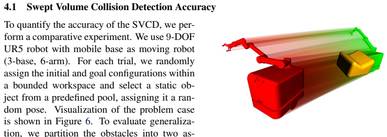
Summary. NeuralSVCD proposes a neural encoder–decoder pipeline for swept-volume collision detection. Each mesh is represented by N sampled surface points with local latent codes and bounding-sphere radii. At inference, a broad phase finds candidate static–moving point pairs and the time t† that minimizes sphere distance along the trajectory; the narrow phase feeds a locally linearized trajectory segment to an MLP decoder, and max-pooling aggregates pair logits. Training uses binary cross-entropy against FCL ground-truth labels with a gradient regularization term. Experiments compare against convex-cell/GJK, sphere/mesh, implicit-function, and discrete/global variants on UR5, ARMADA, and mobile-UR5 tasks, reporting accuracy/runtime trade-offs and motion-planning success rates.
Significance. The paper targets a practical problem and has a clear, plausible architecture. The broad/narrow two-step design with temporal locality is a sensible way to make neural collision prediction continuous, and if the reported gains hold it would be a useful step over sphere- and hull-based SVCD. Strengths include public code and videos, held-out evaluation with in-domain/out-of-domain objects, and integration into a standard optimizer. However, the main accuracy claim rests on an unverified approximation about the pseudo-critical time; the motion-planning comparison varies optimizer hyperparameters across methods; and no uncertainty quantification is provided. These issues are fixable and do not invalidate the approach, but they must be addressed before the paper's claims are fully supported.
major comments (5)
- [§3.2, Eq. (1)] The continuous-accuracy claim in §4.1 (90% at 6.4e-5 s, peak 95.6%) is load-bearing on the assumption that t† ≈ t*. The broad phase minimizes the enclosing-sphere distance with Newton's method, but no initialization or multi-start is described; for spline trajectories with multiple local extrema the optimizer can return a time with no actual mesh contact. Moreover, even the global minimum of sphere separation is not generally the time of maximum mesh penetration for non-convex/thin geometry. The discrete-variant ablation does not isolate t† error. Please report (a) recall of the broad-phase candidate set against ground truth over a dense time grid, and (b) the distribution of |t† - argmax_t f_decoder(t)| on test cases. Without this, the speed/accuracy advantage over continuous GJK/sphere baselines is not established.
- [§3.1] The radius r_i = α min_j dist(p_i, p_j) is asserted to enclose the local geometry near p_i. For concave or elongated Voronoi cells the nearest-representative distance is not a bound on the extent of the local patch, so a truly colliding pair can be absent from the broad-phase candidate set and never reach the decoder; this is a false-negative mechanism distinct from t† error. Please provide a formal condition or a conservative radius computation, and measure broad-phase recall against FCL on the evaluation set.
- [§4.2, Tables 3–5] The claim that cuRobo-NeuralSVCD outperforms cuRobo-sphere with the 'same planner but different collision detectors' is weakened by the fact that optimizer hyperparameters differ across methods within each task: MPPI interpolation 4 vs 100, number of samples 200 vs 50, LBFGS interpolation 2 vs 100/50, control points, and activation distances all vary. Differences in success rate and planning time may be attributable to optimizer tuning rather than the collision detector. Please either keep optimizer hyperparameters fixed across methods, sweep them for all methods, or demonstrate that the conclusion is stable over a range of settings.
- [§4.1, Table 1] All accuracy, runtime, and planning results are single point estimates. No standard deviations, confidence intervals, or significance tests are reported; claims of 'consistently outperforms' and speed-ups (120x–590x, 24x) have no uncertainty attached. Please run multiple seeds (at least for network training and optimizer randomness) and report error bars or paired tests.
- [§6.1] The paper acknowledges that using logits as collision distance is an approximation that can lead optimizers to local minima, but it does not quantify the mismatch. Since the planner cost C_SVCD is built from these logits, the planner results depend on this surrogate. Please add an evaluation of logit quality against penetration depth (e.g., correlation or calibration on the SVCD test set) or compare against a distance-based version of the same collision cost.
minor comments (5)
- [Appendix A] There is a garbled duplicated sentence: 'The training objective is defined as ... However, binary classification loss alone results ... This is undesirable because The training objective is defined as ...' Please rewrite this paragraph.
- [Table 2] The notation U(min, max) with '⊂ R' or '⊂ Z' is confusing; if U denotes a uniform distribution, define it explicitly and distinguish the sampling domain from the sampled values.
- [Algorithm 1] The variable 'ccd output' should be 'SVCD output' for consistency, and the broadPhase function's output is not fully specified with respect to Eq. (1).
- [§3.2] Minor formatting: 'mesh mov and meshstatic' lacks subscript formatting; also the subscript on t† is sometimes omitted, making it hard to distinguish pair-specific times.
- [Figure 5] The axes are not labeled clearly, and the text alternates between 'success rate' and 'accuracy'. Please use consistent terminology and label axes.
Circularity Check
No significant circularity: predictions are trained and evaluated against external FCL ground truth, and the central claims rest on held-out empirical comparison rather than by-construction equivalence.
full rationale
The paper's core SVCD prediction is not defined in terms of its own output. Training uses ground-truth labels ySVCD computed with the external FCL library [24]: 'Ground-truth collision labels ySVCD are computed using the FCL library [24].' The reported accuracy numbers (90% at 6.4e-5 s, peaking at 95.6% in-domain and 94.9% out-of-domain) are then measured on held-out problem instances against the same external ground-truth standard, so the headline accuracy is an empirical result, not a forced consequence of the model's construction. The encoder architecture is taken from the authors' prior FER-VN-OccNet paper [33] and the local-crop collision idea from their prior collision-network paper [5], but these are published architectural and predecessor works with independent content; they are not invoked as a 'uniqueness theorem' forbidding alternatives, and the paper further benchmarks against sphere-based, mesh/GJK, implicit-function, and discrete- and global-representation ablated baselines. The broad-phase pseudo-critical time t† is introduced as an approximation: 'We assume that the pseudo-critical collision time t† sufficiently approximates the true critical collision time t*' (Section 3.2). That is a stated approximation assumption, not a self-referential definition; the same holds for the unproved sphere-enclosure radius choice ri = α min_j dist(pi,pj). These are correctness and robustness risks, not circularity. No fitted parameter is renamed as a prediction, and no equation reduces to its own input by construction. Therefore, under the hard rules, no circular step can be exhibited, and the honest finding is a score of 0.
Axiom & Free-Parameter Ledger
free parameters (3)
- N (number of representative points per mesh)
- alpha (sphere radius multiplier)
- Trajectory interpolation density in neural decoder
axioms (5)
- domain assumption FCL collision labels ySVCD are correct for training and evaluation.
- ad hoc to paper Pseudo-critical time t† approximates true critical time t*.
- ad hoc to paper Logits from fSVCD can serve as collision distance for optimization.
- ad hoc to paper Local linearization around t† captures the relevant swept volume segment.
- domain assumption Encoder FER-VN-OccNet and latent rotation D(R) from [33] preserve rigid-body properties.
Cite this review
Pith. "Pith review of NeuralSVCD for Efficient Swept Volume Collision Detection." pith.science (2026). https://pith.science/paper/226STIS3
@misc{pith2026250900499,
  author       = {Pith},
  title        = {Pith review of: NeuralSVCD for Efficient Swept Volume Collision Detection},
  year         = {2026},
  howpublished = {\url{https://pith.science/paper/226STIS3}},
  note         = {Machine review of arXiv:2509.00499}
}
read the original abstract
Robot manipulation in unstructured environments requires efficient and reliable Swept Volume Collision Detection (SVCD) for safe motion planning. Traditional discrete methods potentially miss collisions between these points, whereas SVCD continuously checks for collisions along the entire trajectory. Existing SVCD methods typically face a trade-off between efficiency and accuracy, limiting practical use. In this paper, we introduce NeuralSVCD, a novel neural encoder-decoder architecture tailored to overcome this trade-off. Our approach leverages shape locality and temporal locality through distributed geometric representations and temporal optimization. This enhances computational efficiency without sacrificing accuracy. Comprehensive experiments show that NeuralSVCD consistently outperforms existing state-of-the-art SVCD methods in terms of both collision detection accuracy and computational efficiency, demonstrating its robust applicability across diverse robotic manipulation scenarios. Code and videos are available at https://neuralsvcd.github.io/.
Figures




Reference graph
Works this paper leans on
-
[1]
C. Ericson. Real-Time Collision Detection. CRC Press, 2004
work page 2004
-
[2]
P. G. Xavier. Fast swept-volume distance for robust collision detection. In Proceedings of International Conference on Robotics and Automation , volume 2, pages 1162–1169. IEEE, 1997
work page 1997
-
[3]
J. Schulman, J. Ho, A. X. Lee, I. Awwal, H. Bradlow, and P. Abbeel. Finding locally opti- mal, collision-free trajectories with sequential convex optimization. In Robotics: science and systems, volume 9, pages 1–10. Berlin, Germany, 2013
work page 2013
-
[4]
E. G. Gilbert, D. W. Johnson, and S. S. Keerthi. A fast procedure for computing the distance between complex objects in three-dimensional space. IEEE Journal on Robotics and Automa- tion, 4(2):193–203, 2002
work page 2002
-
[5]
D. Son and B. Kim. Local object crop collision network for efficient simulation of non-convex objects in gpu-based simulators. arXiv preprint arXiv:2304.09439, 2023
work page internal anchor Pith review Pith/arXiv arXiv 2023
-
[6]
B. Sundaralingam, S. K. S. Hari, A. Fishman, C. Garrett, K. Van Wyk, V . Blukis, A. Millane, H. Oleynikova, A. Handa, F. Ramos, et al. Curobo: Parallelized collision-free robot motion 9 generation. In 2023 IEEE International Conference on Robotics and Automation (ICRA), pages 8112–8119. IEEE, 2023
work page 2023
-
[7]
C. W. Ramsey, Z. Kingston, W. Thomason, and L. E. Kavraki. Collision-affording point trees: Simd-amenable nearest neighbors for fast collision checking. arXiv preprint arXiv:2406.02807, 2024
work page internal anchor Pith review Pith/arXiv arXiv 2024
-
[8]
S. Sui, L. Sentis, and A. Bylard. Hardware-accelerated ray tracing for discrete and continuous collision detection on gpus. arXiv preprint arXiv:2409.09918, 2024
work page internal anchor Pith review Pith/arXiv arXiv 2024
- [9]
- [10]
-
[11]
J. Canny. Collision detection for moving polyhedra. IEEE Transactions on Pattern Analysis and Machine Intelligence, (2):200–209, 1986
work page 1986
- [12]
-
[13]
S. Redon, A. Kheddar, and S. Coquillart. An algebraic solution to the problem of collision detection for rigid polyhedral objects. In Proceedings 2000 ICRA. Millennium Conference. IEEE International Conference on Robotics and Automation. Symposia Proceedings (Cat. No. 00CH37065), volume 4, pages 3733–3738. IEEE, 2000
work page 2000
-
[14]
M. Tang, Y . J. Kim, and D. Manocha. C2a: Controlled conservative advancement for con- tinuous collision detection of polygonal models. In 2009 IEEE International Conference on Robotics and Automation, pages 849–854. IEEE, 2009
work page 2009
-
[15]
M. Peternell, H. Pottmann, T. Steiner, and H. Zhao. Swept volumes. Computer-Aided Design and Applications, 2(5):599–608, 2005
work page 2005
-
[16]
J. Rossignac, J. J. Kim, S. Song, K. Suh, and C. Joung. Boundary of the volume swept by a free-form solid in screw motion. Computer-Aided Design, 39(9):745–755, 2007
work page 2007
-
[17]
S. Abrams and P. K. Allen. Computing swept volumes. The Journal of Visualization and Computer Animation, 11(2):69–82, 2000
work page 2000
-
[18]
Y . J. Kim, G. Varadhan, M. C. Lin, and D. Manocha. Fast swept volume approximation of complex polyhedral models. In Proceedings of the eighth ACM symposium on Solid modeling and applications, pages 11–22, 2003
work page 2003
- [19]
-
[20]
S. Sell ´an, N. Aigerman, and A. Jacobson. Swept volumes via spacetime numerical continua- tion. ACM Transactions on Graphics (TOG), 40(4):1–11, 2021
work page 2021
-
[21]
D. Son, H. Yang, and D. Lee. Sim-to-real transfer of bolting tasks with tight tolerance. In 2020 IEEE/RSJ International Conference on Intelligent Robots and Systems (IROS) , pages 9056–9063. IEEE, 2020
work page 2020
-
[22]
M. Danielczuk, A. Mousavian, C. Eppner, and D. Fox. Object rearrangement using learned im- plicit collision functions. In 2021 IEEE International Conference on Robotics and Automation (ICRA), pages 6010–6017. IEEE, 2021. 10
work page 2021
-
[23]
H. Wang, S. Sridhar, J. Huang, J. Valentin, S. Song, and L. J. Guibas. Normalized object coordinate space for category-level 6d object pose and size estimation. InThe IEEE Conference on Computer Vision and Pattern Recognition (CVPR) , June 2019
work page 2019
-
[24]
J. Pan, S. Chitta, and D. Manocha. Fcl: A general purpose library for collision and proximity queries. In 2012 IEEE international conference on robotics and automation, pages 3859–3866. IEEE, 2012
work page 2012
-
[25]
J. Kim, J. Kim, D. Lee, Y . Jang, and B. Kim. Design of a low-cost and lightweight 6 dof bimanual arm for dynamic and contact-rich manipulation. arXiv preprint arXiv:2502.16908 , 2025
work page internal anchor Pith review Pith/arXiv arXiv 2025
-
[26]
M. Z. Irshad, S. Zakharov, R. Ambrus, T. Kollar, Z. Kira, and A. Gaidon. Shapo: Implicit representations for multi-object shape, appearance, and pose optimization. In European Con- ference on Computer Vision, pages 275–292. Springer, 2022
work page 2022
-
[27]
Y . Hong, K. Zhang, J. Gu, S. Bi, Y . Zhou, D. Liu, F. Liu, K. Sunkavalli, T. Bui, and H. Tan. Lrm: Large reconstruction model for single image to 3d. arXiv preprint arXiv:2311.04400 , 2023
Pith/arXiv arXiv 2023
- [28]
-
[29]
G. Williams, P. Drews, B. Goldfain, J. M. Rehg, and E. A. Theodorou. Aggressive driving with model predictive path integral control. In 2016 IEEE international conference on robotics and automation (ICRA), pages 1433–1440. IEEE, 2016
work page 2016
-
[30]
D. C. Liu and J. Nocedal. On the limited memory bfgs method for large scale optimization. Mathematical programming, 45(1):503–528, 1989
1989
-
[31]
H. J. T. Suh, T. Pang, and R. Tedrake. Bundled gradients through contact via randomized smoothing. IEEE Robotics and Automation Letters , 7(2):4000–4007, 2022
work page 2022
-
[32]
C. R. Qi, H. Su, K. Mo, and L. J. Guibas. Pointnet: Deep learning on point sets for 3d classification and segmentation. In Proceedings of the IEEE conference on computer vision and pattern recognition, pages 652–660, 2017
2017
-
[33]
D. Son, J. Kim, S. Son, and B. Kim. An intuitive multi-frequency feature representation for SO(3)-equivariant networks. In The Twelfth International Conference on Learning Represen- tations, 2024. URL https://openreview.net/forum?id=5JWAOLBxwp
work page 2024
-
[34]
O. Puny, M. Atzmon, E. J. Smith, I. Misra, A. Grover, H. Ben-Hamu, and Y . Lipman. Frame averaging for invariant and equivariant network design. InInternational Conference on Learn- ing Representations, 2022. URL https://openreview.net/forum?id=zIUyj55nXR
work page 2022
-
[35]
J. Yang, C. Deng, J. Wu, R. Antonova, L. Guibas, and J. Bohg. Equivact: Sim (3)-equivariant visuomotor policies beyond rigid object manipulation. In 2024 IEEE international conference on robotics and automation (ICRA) , pages 9249–9255. IEEE, 2024. 11 A Implementation Details in training From given training datasetD, the training objective isP d∈D LSV CD(...
work page 2024
-
[36]
We also modify the calculating gradient during L-BFGS to be the bundled gradient [31], which 13 Figure 8: Illustration of pre-processing for achieving invariance. Case 1 and 2 have the same relative transform between two objects, but their global transforms are different. If we treat the two objects as a single composite rigid body, we can assign frames {...
-
[37]
Let the combined input be x = [ξ; z1; z2; p1; p2]. We define the preprocessing function as Φ(x) = 1 max(∥z1∥, ∥z2∥) (ϕ(x)−1 · x), with ϕ : RM → SE (3) such that ϕ(T · x) = T · ϕ(x) ∀T ∈ SE (3), where M is the dimension of x and ∥z∥ is Euclidean norm of z. It is straightforward to verify that Φ is invariant under any transformation in SE (3) and scale. We ...
work page 2000
This paper was first reviewed by deepseek-v4-flash on August 5, 2026.
discussion (0)
Sign in with ORCID, Apple, or X to comment. Anyone can read and Pith papers without signing in.