REVIEW 4 major objections 6 minor 32 references
The Optimiser Hidden in Plain Sight: Training with the Loss Landscape's Induced Metric
T0 review · 4 major / 6 minor · reviewed 2026-08-05 · deepseek-v4-flash
Pith's one-line read Using the loss landscape's induced Riemannian metric as a gradient preconditioner yields optimizers that shrink steps in steep regions and, in one RMSprop-based variant, slightly beat Adam and AdamW on average.
desk verdict The geometry is neat and the code ships, but the central curvature-adaptivity claim doesn't hold up; treat this as a well-tested normalized-gradient variant, not a curvature-adaptive method. read the letter →
The pith
A machine-rendered reading of the paper's core claim, the machinery that carries it, and where it could break.
The reading
What carries the argument
The induced (pull-back) metric g_ij = γ_ij + l_i l_j on the loss-surface graph, inverted by a rank-one update of γ^{-1}. It does the work: the denominator 1 + Σ γ^{kl} l_k l_l is a scalar computed by one dot product, converting gradient magnitude into a per-step shrinkage factor while preserving the descent direction set by the ambient geometry.
What would settle it
Train on a strictly linear loss L(θ)=a·θ, whose curvature is exactly zero but whose gradient norm ‖a‖ is large. Equation 13 still multiplies the update by 1/(1+ξ‖a‖²), so the claimed curvature-adaptive shrinkage is visibly just gradient-norm clipping. The converse check is a sharply curved quadratic centered near zero with a small gradient: the formula gives almost no shrinkage, contradicting the claim that high curvature triggers smaller steps.
Extended reading notes
Core claim
Embed the loss surface as the graph L = f(L(θ)) in an ambient space with coordinates (θ, L) and a metric that is block-diagonal, with any chosen parameter metric γ in the horizontal block and 1 in the vertical block. Pulling this metric back to parameter space gives g_ij = γ_ij + (∂L/∂θ_i)(∂L/∂θ_j). Inverting via the rank-one update formula for a matrix plus an outer product and using the inverse metric to precondition gradient descent yields δθ_i = −η Σ_j γ^{ij} (∂L/∂θ_j) / (1 + Σ_{k,l} γ^{kl} (∂L/∂θ_k)(∂L/∂θ_l)). With diagonal γ this is the base gradient divided by one plus a scaled squared gradient norm, so the step shrinks where the gradient is large without rotating the direction of ste
Load-bearing premise
The load-bearing premise is that the squared gradient norm measures local curvature, together with the choice that the ambient metric's vertical component is 1 (which fixes the loss scale); if the gradient is large on a flat but sloped surface, the 'automatic' shrinkage is actually controlled by the free parameter ξ rather than by geometry.
Editorial extensions
If this is right
- Updates follow Eq. 13: divide the gradient by 1 + ξ Σ (∂L/∂θ_i)², so a single scalar dot product converts gradient magnitude into automatic step-size reduction at O(N) cost per step, matching Adam.
- The framework is a wrapper: replacing γ with the metric implied by any preconditioner such as RMSprop or Muon induces an optimizer with the same shrinkage property, and standard SGD and AdamW are recovered as ξ→0 limits.
- Decoupled weight decay is the geometrically natural regularizer, so no ad-hoc coupling is needed.
- The log-loss embedding f(L) = ln L produces a learning-rate-schedule-like behavior with warm-up and decay phases, tying scheduling to the loss magnitude itself.
- Empirically, the RMS-metric variant achieved the best average validation performance on the regression and TinyShakespeare tasks and the best single-run accuracy on CIFAR-10, while the log-loss variant was the only optimizer to solve all tested low-dimensional benchmark functions.
Reading between the lines
- Because the shrinkage factor is global, one outlier gradient component can suppress the whole update; a per-layer or per-block normalization of Σ l_k² would be a natural testable extension.
- The paper's claimed tie between gradient norm and curvature can be checked directly: on a linear loss (zero curvature, large gradient) the update still shrinks by 1/(1+ξ‖∇L‖²), so in that regime the effect is indistinguishable from plain gradient clipping.
- The log-loss variant's erratic transfer between low and high dimensions hints that loss-scale dynamics, not geometry alone, drive its success; testing on losses with a lower bound or on reinforcement-learning returns would separate those effects.
- If the geometric derivation is the real source of the gains, embedding the loss into more than one extra dimension—for instance, one vertical coordinate per loss term—should change optimizer behavior in predictable ways; this is directly testable and could yield multi-objective optimizers.
Signed reviews
Editorial analysis
A structured set of objections, weighed in public.
Referee Report
Summary. The paper proposes a new class of optimizers derived from the Riemannian pull-back metric obtained by embedding the loss function as a graph over parameter space. For an ambient metric with identity horizontal part, the Sherman–Morrison formula gives the inverse metric and leads to the update δθ_i = -η ∂L/∂θ_i / (1 + ξ Σ_k (∂L/∂θ_k)^2) (Eq. 13). Variants using a log-loss embedding and an RMSprop-based ambient metric are also proposed. The paper benchmarks these optimizers against SGD, Adam, AdamW, and Muon on five low-dimensional test functions, an MLP regression task, MNIST MLP classification, ResNet-18 on CIFAR-10, and a TinyShakespeare transformer language task. Claims include automatic step-size reduction in regions of high curvature, natural appearance of decoupled weight decay and a scheduled learning rate, and slight empirical improvement of the RMS variant over Adam/AdamW.
Significance. The manuscript's strengths are its transparent algebraic derivation, a relatively broad set of benchmarks, and the provision of JAX/PyTorch code. If the geometric framing were fully established, the connection between loss-landscape visualization and optimization would be a useful perspective, and the algorithms are indeed cheap (O(N) per step). However, the central theoretical claim that the method adapts to curvature is not supported by the equations, and the reported empirical gains are smaller than the run-to-run variability. The framework may still be of interest as a smooth, global gradient-norm clipping scheme, but the current text overstates what has been rigorously shown.
major comments (4)
- [Abstract, §2 Eq. (13)] The statement that the effective learning rate is 'automatically decreased in regions of high curvature' is not supported. The prefactor in Eq. (13) is 1/(1+ξΣ_k(∂L/∂θ_k)^2), which depends only on first derivatives and is a single global scalar for all coordinates. On L = 0.5 a θ², the denominator is largest far from the minimum even though the curvature a is constant; at a saddle point ∇L = 0, so no adaptation occurs despite possibly large Hessian eigenvalues. Eq. (13) is therefore a global gradient-norm rescaling, not a curvature-adaptive preconditioner. The text should be reworded to 'large-gradient' or 'steep-slope' regions, and any curvature claim should be either removed or separately motivated by additional analysis.
- [Algorithm 1 line 12, Algorithm 2 line 13, Appendix listing] The pseudocode writes the weight-decay update as θ_t ← θ_{t−1} − η r_t m̂_t + λθ_{t−1}, which adds λθ_{t−1}. The shipped code in the appendix (lines 125, 208, 308) implements updates = -lr * metric_scale * m / (...) - lr * weight_decay * p, i.e., subtraction. Since the experiments are run with the code, the pseudocode does not describe the evaluated method. This discrepancy must be fixed and the sign/direction of weight decay clarified before the results are reproducible from the paper alone.
- [§2 Eq. (5), Eq. (13)] The vertical metric component is set to 1 with the statement that its value 'can be absorbed into the normalisation of the loss function.' This is only partly true for the update: under L → cL, the denominator in Eq. (13) becomes 1 + ξ c² Σ(∂L)^2 unless ξ is rescaled. Thus the effective clipping threshold depends on the arbitrary normalization of the loss, and the claimed 'automatic' adaptivity is not scale-invariant. The paper should state explicitly that ξ absorbs the loss scale, which weakens the geometric interpretation of the clipping scale.
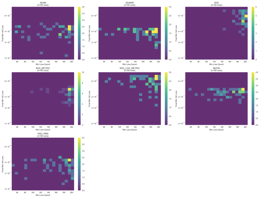
- [§3.3–3.5, Tables 3–4] The conclusion that one variant 'demonstrated slight improvement on average over Adam and AdamW' is not supported by the reported statistics. For CIFAR-10, SGD RMS has mean max validation accuracy 0.8263 ± 0.0217 versus Adam's 0.8260 ± 0.0210; for TinyShakespeare, SGD RMS has min validation perplexity 4.4328 ± 0.0437 versus AdamW's 4.4372 ± 0.0397. These differences are far smaller than one standard deviation, no significance or paired comparisons are provided, and selecting the best 50 of 200–500 Bayesian-sweep runs can inflate apparent differences. Please report paired significance tests or honest error bars, and either qualify the claim as 'competitive' or provide stronger statistical evidence for 'improvement'.
minor comments (6)
- [§2 Eq. (6)] Including f(L) on the right-hand side of the gradient-flow equation is introduced as 'the author's choice, and not fundamental.' This is a substantial modeling choice; a geometric derivation or at least a more principled justification would strengthen the paper.
- [Algorithm 1 line 11, Appendix] The pseudocode applies bias correction of momentum inside γ^{-1}, while the code applies it after forming the tree_map update. Please clarify the exact ordering in the implementation so the pseudocode matches the code.
- [§2 before Eq. (8)] The symbol l_i is used for both γ^{ij} l_j and ∂L/∂θ_i. This is confusing; use a different notation for the raised-index object.
- [§2 bullet 'Only one new hyperparameter'] In batched training, the EMA decay β is a second new hyperparameter; the sentence should be qualified to the non-batched case or to the case where β is fixed.
- [§3.1] The text claims custom optimizers were 'typically' fastest, but on Rastrigin SGD is fastest. The main text acknowledges this; the figure captions and summary should be more consistent about wall-time versus iteration counts.
- [§3.3] The protocol for choosing the 'best 50' runs from the hyperparameter sweeps should be stated (e.g., based on final validation metric, or best validation during training?). This is important for interpreting the distributions.
Circularity Check
No significant circularity: the update rule is derived by direct algebra from the stated pull-back metric, and the empirical benchmarks are external rather than back-fitted. The main weakness is an unsupported interpretation of gradient-norm rescaling as curvature adaptation, which is a correctness concern, not a circular input.
full rationale
The derivation chain is self-contained: Eq. 5 defines the ambient metric with a unit vertical component, Eq. 7 defines the pull-back metric as g_ij = γ_ij + ∂_i L ∂_j L, Eq. 8 applies Sherman-Morrison to invert it, and Eq. 10 (specializing to Eq. 13) follows by direct substitution into the preconditioned gradient-flow equation. No parameter is fitted to the benchmark data and then relabelled as a prediction; the reported comparisons to Adam, AdamW, SGD, and Muon are external empirical evaluations. The only self-citation is the GitHub implementation repository (ref [19]), which is code and is not load-bearing for any theoretical claim. The paper explicitly acknowledges its two free choices: the unit vertical metric component (Eq. 5: 'its value can be absorbed into the normalisation of the loss function') and the inclusion of f(L) in the flow equation (Eq. 6: 'this is the author’s choice, and not fundamental'). These are admitted ansätze, not hidden circular inputs. The main critique is interpretive: Eq. 13's denominator is 1 + ξΣ(∂L)^2, a global gradient-norm rescaling, and the paper's assertion that this quantity measures 'local curvature' is unsupported by any curvature invariant. That undercuts the strength of the theoretical selling point, but it is a correctness/rigour objection about the proxy, not a demonstration that the result was assumed in its own input. Therefore no circularity is present; the derivation is algebraically honest even where the interpretation is overstated.
Assumptions & free parameters
free parameters (4)
- ξ (metric coefficient) =
tuned per task; paper suggests ξ ~ 1/N
- β (EMA decay for metric denominator) =
tuned per task, default 0.8 in code
- β_rms (EMA decay for RMS variant) =
tuned per task, default 0.99 in code
- Loss scale / normalization =
arbitrary, absorbed into ξ
assumptions (8)
- standard math Sherman-Morrison formula for rank-one update of a matrix inverse
- standard math Riemannian geometry: metric, pull-back, gradient flow on a manifold
- ad hoc to paper The ambient metric is block diagonal with vertical component 1
- domain assumption Loss landscape is a smooth graph L = f(L(θ))
- domain assumption f is monotonic and, for the log variant, L > 0
- ad hoc to paper Including f(L) on the RHS of gradient flow (Eq. 6)
- domain assumption EMA of squared gradient norms approximates the batch metric
- ad hoc to paper The squared gradient norm is a proxy for local curvature
Cite this review
Pith. "Pith review of The Optimiser Hidden in Plain Sight: Training with the Loss Landscape's Induced Metric." pith.science (2026). https://pith.science/paper/FL77OHW3
@misc{pith2026250903594,
  author       = {Pith},
  title        = {Pith review of: The Optimiser Hidden in Plain Sight: Training with the Loss Landscape's Induced Metric},
  year         = {2026},
  howpublished = {\url{https://pith.science/paper/FL77OHW3}},
  note         = {Machine review of arXiv:2509.03594}
}
read the original abstract
We present a class of novel optimisers for training neural networks that makes use of the Riemannian metric naturally induced when the loss landscape is embedded in higher-dimensional space. This is the same metric that underlies common visualisations of loss landscapes. By taking this geometric perspective literally and using the induced metric, we develop a new optimiser and compare it to existing methods, namely: SGD, Adam, AdamW, and Muon, across a range of tasks and architectures. Empirically, we conclude that this new class of optimisers is highly effective in low dimensional examples, and provides slight improvement over state-of-the-art methods for training neural networks. These new optimisers have theoretically desirable properties. In particular, the effective learning rate is automatically decreased in regions of high curvature acting as a smoothed out form of gradient clipping. Similarly, one variant of these optimisers can also be viewed as inducing an effective scheduled learning rate and decoupled weight decay is the natural choice from our geometric perspective. The basic method can be used to modify any existing preconditioning method. The new optimiser has a computational complexity comparable to that of Adam.
Figures


Figures from the paper (10 more)




Reference graph
Works this paper leans on
-
[1]
Visualizing the loss landscape of neural nets,
H. Li, Z. Xu, G. Taylor, C. Studer, and T. Goldstein, “Visualizing the loss landscape of neural nets,” Advances in neural information processing systems31 (2018)
work page 2018
-
[2]
On the difficulty of training recurrent neural networks,
R. Pascanu, T. Mikolov, and Y. Bengio, “On the difficulty of training recurrent neural networks,” in International conference on machine learning, pp. 1310–1318, Pmlr. 2013
work page 2013
-
[3]
Accurate, large minibatch sgd: Training imagenet in 1 hour,
P. Goyal, P. Doll´ ar, R. Girshick, P. Noordhuis, L. Wesolowski, A. Kyrola, A. Tulloch, Y. Jia, and K. He, “Accurate, large minibatch sgd: Training imagenet in 1 hour,” arXiv preprint arXiv:1706.02677(2017)
arXiv 2017
-
[4]
Sgdr: Stochastic gradient descent with warm restarts,
I. Loshchilov and F. Hutter, “Sgdr: Stochastic gradient descent with warm restarts,” arXiv preprint arXiv:1608.03983(2016)
arXiv 2016
-
[5]
Decoupled weight decay regularization,
I. Loshchilov and F. Hutter, “Decoupled weight decay regularization,” arXiv preprint arXiv:1711.05101(2017)
arXiv 2017
-
[6]
Muon: An optimizer for hidden layers in neural networks,
K. Jordan, Y. Jin, V. Boza, J. You, F. Cesista, L. Newhouse, and J. Bernstein, “Muon: An optimizer for hidden layers in neural networks,” 2024. https://kellerjordan.github.io/posts/muon/
work page 2024
-
[7]
Muon is scalable for llm training,
J. Liu, J. Su, X. Yao, Z. Jiang, G. Lai, Y. Du, Y. Qin, W. Xu, E. Lu, J. Yan, et al., “Muon is scalable for llm training,” arXiv preprint arXiv:2502.16982(2025)
arXiv 2025
-
[8]
Gradient-based learning applied to document recognition,
Y. Lecun, L. Bottou, Y. Bengio, and P. Haffner, “Gradient-based learning applied to document recognition,” Proceedings of the IEEE86 no. 11, (1998) 2278–2324
work page 1998
Show all 32 references
-
[9]
Deep residual learning for image recognition,
K. He, X. Zhang, S. Ren, and J. Sun, “Deep residual learning for image recognition,” in Proceedings of the IEEE conference on computer vision and pattern recognition, pp. 770–778. 2016
2016
-
[10]
Learning multiple layers of features from tiny images.(2009),
A. Krizhevsky, G. Hinton, et al., “Learning multiple layers of features from tiny images.(2009),” 2009
2009
-
[11]
Attention is all you need,
A. Vaswani, N. Shazeer, N. Parmar, J. Uszkoreit, L. Jones, A. N. Gomez, L. Kaiser, and I. Polosukhin, “Attention is all you need,” 2017. https://arxiv.org/pdf/1706.03762.pdf
2017 arXiv
-
[12]
Optimization by simulated annealing,
S. Kirkpatrick, C. D. Gelatt, and M. P. Vecchi, “Optimization by simulated annealing,” Science 220 no. 4598, (1983) 671–680, https://www.science.org/doi/pdf/10.1126/science.220.4598.671. 36
1983 doi
-
[13]
Stochastic gradient hamiltonian monte carlo,
T. Chen, E. Fox, and C. Guestrin, “Stochastic gradient hamiltonian monte carlo,” in International conference on machine learning, pp. 1683–1691, PMLR. 2014
2014
-
[14]
Born-Infeld (BI) for AI: Energy-Conserving Descent (ECD) for Optimization,
G. B. De Luca and E. Silverstein, “Born-Infeld (BI) for AI: Energy-Conserving Descent (ECD) for Optimization,” PMLR 162 (2022) 4918, arXiv:2201.11137 [cs.LG]
2022 arXiv
-
[15]
Bayesian learning via stochastic gradient langevin dynamics,
M. Welling and Y. W. Teh, “Bayesian learning via stochastic gradient langevin dynamics,” in Proceedings of the 28th international conference on machine learning (ICML-11), pp. 681–688. 2011
2011
-
[16]
Absil, R
P. Absil, R. Mahony, and R. Sepulchre, Optimization Algorithms on Matrix Manifolds. Princeton University Press, 2009. https://books.google.com/books?id=NSQGQeLN3NcC
2009
-
[17]
A survey of geometric optimization for deep learning: from euclidean space to riemannian manifold,
Y. Fei, Y. Liu, C. Jia, Z. Li, X. Wei, and M. Chen, “A survey of geometric optimization for deep learning: from euclidean space to riemannian manifold,” ACM Computing Surveys57 no. 5, (2025) 1–37
2025
-
[18]
The unreasonable effectiveness of recurrent neural networks
A. Karpathy, “The unreasonable effectiveness of recurrent neural networks.” Blog post, 2015. http://karpathy.github.io/2015/05/21/rnn-effectiveness/
2015
-
[19]
Induced metric repository
T. R. Harvey, “Induced metric repository.” https://github.com/harveyThomas4692/Induced-Metric-Optimiser
-
[20]
JAX: composable transformations of Python+NumPy programs,
J. Bradbury, R. Frostig, P. Hawkins, M. J. Johnson, C. Leary, D. Maclaurin, G. Necula, A. Paszke, J. VanderPlas, S. Wanderman-Milne, and Q. Zhang, “JAX: composable transformations of Python+NumPy programs,” 2018. http://github.com/jax-ml/jax
2018
-
[21]
Pytorch: An imperative style, high-performance deep learning library,
A. Paszke, S. Gross, F. Massa, A. Lerer, J. Bradbury, G. Chanan, T. Killeen, Z. Lin, N. Gimelshein, L. Antiga, et al., “Pytorch: An imperative style, high-performance deep learning library,” Advances in neural information processing systems32 (2019)
2019
-
[22]
Natural gradient works efficiently in learning,
S.-i. Amari, “Natural gradient works efficiently in learning,” Neural Computation 10 no. 2, (1998) 251–276
1998
-
[23]
Natural gradient methods: Perspectives, efficient-scalable approximations, and analysis,
R. Shrestha, “Natural gradient methods: Perspectives, efficient-scalable approximations, and analysis,” arXiv preprint arXiv:2303.05473(2023)
2023 arXiv
-
[24]
Neural networks for machine learning
G. Hinton, N. Srivastava, and K. Swersky, “Neural networks for machine learning.” Coursera, lecture 6.5, 2012. University of Toronto. 37
2012
-
[25]
Adjustment of an inverse matrix corresponding to a change in one element of a given matrix,
J. Sherman and W. J. Morrison, “Adjustment of an inverse matrix corresponding to a change in one element of a given matrix,” The Annals of Mathematical Statistics20 (1949) 621
1949
-
[26]
Scaling laws for neural language models,
J. Kaplan, S. McCandlish, T. Henighan, T. B. Brown, B. Chess, R. Child, S. Gray, A. Radford, J. Wu, and D. Amodei, “Scaling laws for neural language models,” arXiv preprint arXiv:2001.08361(2020)
2001 arXiv
-
[27]
Deep learning scaling is predictable, empirically,
J. Hestness, S. Narang, N. Ardalani, G. Diamos, H. Jun, H. Kianinejad, M. M. A. Patwary, Y. Yang, and Y. Zhou, “Deep learning scaling is predictable, empirically,” arXiv preprint arXiv:1712.00409(2017)
2017 arXiv
-
[28]
Some methods of speeding up the convergence of iteration methods,
B. T. Polyak, “Some methods of speeding up the convergence of iteration methods,” Ussr computational mathematics and mathematical physics4 no. 5, (1964) 1–17
1964
-
[29]
A literature survey of benchmark functions for global optimisation problems,
M. Jamil and X.-S. Yang, “A literature survey of benchmark functions for global optimisation problems,” International Journal of Mathematical Modelling and Numerical Optimisation4 no. 2, (2013) 150–194
2013
-
[30]
An automatic method for finding the great- est or least value of a function,
H. H. Rosenbrock, “An automatic method for finding the great- est or least value of a function,”The Computer Journal3 no. 3, (01, 1960) 175–184, https://academic.oup.com/comjnl/article-pdf/3/3/175/988633/030175.pdf
1960
-
[31]
Gaussian error linear units (gelus),
D. Hendrycks and K. Gimpel, “Gaussian error linear units (gelus),” arXiv preprint arXiv:1606.08415(2016)
2016 arXiv
-
[32]
Taking the human out of the loop: A review of bayesian optimization,
B. Shahriari, K. Swersky, Z. Wang, R. P. Adams, and N. de Freitas, “Taking the human out of the loop: A review of bayesian optimization,” Proceedings of the IEEE 104 no. 1, (2016) 148–175. 38
2016
Reviewed August 5, 2026 · model on record in the stance chip above.
Discussion (0). Continue with ORCID to comment.