REVIEW 4 major objections 3 minor 1 cited by
End-to-end simulations show RISTRETTO can detect Proxima b in reflected light in about 55 hours, and its O2 and H2O signatures in about 85 hours.
Reviewed by Pith at T0; open to challenge. T0 means a machine referee read the full paper against a public rubric. the ladder, T0–T4 →
End-to-end simulations forecast that RISTRETTO can detect Proxima b in reflected light in 55 hours and constrain its albedo to 20%, with molecular features emerging near 85 hours under an Earth-like atmosphere assumption.
T0 review reviewed 2026-08-04 challenge →
load-bearing objection A careful simulation that makes the 55-hour planet detection credible, but the abstract's 85-hour O2/H2O claim is a matched-filter upper bound, and H2O is not detected by the simpler molecular model even at 100 hours. the 4 major comments →
Simulating RISTRETTO: Proxima b detectability in reflected light
The pith
A machine-rendered reading of the paper's core claim, the machinery that carries it, and where it could break.
The reading
Core claim
The central claim is that RISTRETTO can detect Proxima b's reflected light at high significance in 55 hours (best 50 hours retained) when the planet has an Earth-like N2-O2 atmosphere with 400 ppm CO2 and a water-covered surface. The detection criterion is 20% precision on the planet-to-star flux ratio, a stricter requirement than simple detection; at this exposure the log-Bayes factor favoring a constant-albedo planet model over a no-planet model averages 10.5, and the recovered inclination and flux ratio match the simulated values aside from a systematic ~20% underestimate caused by setting the planet-position coupling ratio to unity in the model. With 80-85 hours the full simulated albedo
What carries the argument
The observable that carries the detection is the normalized long-to-short exposure ratio of each echelle order (one spectral strip of the cross-dispersed format), Eq. 8, which removes broadband telluric and instrumental transmission; in that ratio the planet appears as the stellar spectrum Doppler-shifted by the planet's orbital motion and scaled by the albedo, phase function, radius ratio, and the ratio of IFU coupling efficiencies. The load-bearing instrument quantity is the simulated coupling curve of the coronagraphic IFU: off-axis fibers suppress the stellar halo to a few × 10^-4 while retaining 30-50% coupling for the planet. The spin-axis technique exploits the steep radial gradient o
Load-bearing premise
The simulated XAO-plus-coronagraph coupling curves, especially off-axis stellar-halo suppression of about 1e-4 and 30-50% planet coupling, faithfully represent the real RISTRETTO front end; required exposure times scale roughly with the inverse square of the achieved planet-to-halo contrast.
What would settle it
Measure the actual off-axis stellar-halo coupling and planet coupling of the RISTRETTO front end on sky under median seeing (0.76 arcsec) and elevation 43 degrees: if the off-axis halo coupling is double the simulated few × 10^-4, the 55-hour forecast becomes roughly 220 hours. Alternatively, a first-light campaign that does not detect Proxima b at the predicted 20%-albedo precision after 100 hours, or detects it at a significantly different inclination or flux ratio, would rule out the simulated Earth-like scenario or the coupling model.
If this is right
- 55 hours of RISTRETTO time would turn Proxima b from a radial-velocity signal into a measured inclination, true mass, and 20%-precision broadband albedo, breaking the Mp sin i degeneracy.
- 85 hours would make the reflected spectrum informative enough to claim molecular absorption by O2 and H2O for an Earth-like planet, the first such measurement for a temperate rocky exoplanet.
- The stellar spin-axis method constrains the ascending node to ±5.4 degrees, enabling a single IFU orientation and halving the needed exposure time for aligned systems; it also yields the stellar inclination through the RV semi-amplitude.
- The restrictive observing constraints (seeing < 0.97 arcsec, airmass < 1.7) still leave about 241 usable hours in a season, so the 55-hour detection is schedulable in one year.
- The same instrument can detect easier targets in a few hours to a few nights, so the methodology generalizes beyond Proxima b to a small sample of nearby gas giants, Neptunes, and super-Earths.
Where Pith is reading between the lines
- If the real on-sky off-axis halo suppression is a factor of two worse than the simulated few × 10^-4 coupling, the 55-hour and 85-hour forecasts would roughly quadruple; the first engineering run should measure the coupling maps directly.
- The normalized-ratio and differential-limb-coupling techniques are transferable to ELT-class instruments, so the paper effectively rehearses the observing and analysis scheme for reflected-light spectroscopy of Earth analogs at larger apertures.
- The spin-orbit alignment assumption is testable: if the stellar spin axis and orbit are misaligned, the method would still measure the stellar inclination but would not fix the ascending node, and the 30-degree-rotated double-exposure strategy would remain necessary.
- By fitting a phase function, the same data could probe orbital phase dependence; observations closer to superior conjunction trade increased reflected flux against smaller angular separation, and the paper's fixed 90-degree-phase assumption likely brackets what is achievable.
Editorial analysis
A structured set of objections, weighed in public.
Referee Report
Summary. The paper presents end-to-end simulations of the proposed RISTRETTO instrument observing Proxima b in reflected light. The authors generate synthetic stellar and planetary spectra, model AO/coronagraph/IFU coupling functions from prior work, propagate the spectra through the PyEchelle spectrograph simulator, and apply a Bayesian nested-sampling framework to a normalized long-exposure/short-exposure ratio. They fit five planet models of increasing complexity. The central quantitative claims are that Proxima b can be detected with a constant-albedo model in about 55 hours of observing time (50 usable hours), reaching ~20% precision on the planet-to-star flux ratio, and that molecular absorption by O2 and H2O can be detected in about 85 hours. A separate section develops a method to constrain the stellar spin-axis orientation using differential coupling in the central single-mode fiber.
Significance. If the 55-hour detection claim holds, this is a significant result: it quantifies a plausible path to the first reflected-light spectroscopy of a temperate rocky exoplanet with a VLT-class instrument, and it introduces a data-analysis methodology that is largely independent of the assumed planetary spectrum. The spin-axis orientation method (Sec. 6) is innovative and is tested over ten noise realizations with consistent recovery of the input angle. The authors are also transparent about several limitations, including the in-sample nature of the full-albedo fit and the omission of the third coupling-function ratio. However, the abstract's molecular-detection claim is not supported by the paper's own results, and the 85-hour figure is a matched-filter upper bound rather than a demonstrated detection of O2 and H2O.
major comments (4)
- [Abstract; Sec. 5.2.4; Sec. 7.1] The abstract states that 'molecular absorption by O2 and H2O can be detected in about 85 hours of observations.' This is internally inconsistent with Sec. 5.2.4, where the HITRAN-based molecular model gives Delta ln Z close to zero for H2O after 100 hours (Appendix C.2), and with Sec. 7.1, which says H2O 'could be detectable with exposure times exceeding 100 hours.' The 85-hour value in Fig. 19 is obtained from the full-albedo model, not from an O2/H2O-specific detection. Please remove the H2O claim from the abstract, or explicitly condition it on an a priori known albedo template.
- [Sec. 4.3.3; Sec. 5.2.3] The 'full albedo spectrum' model is an in-sample matched filter: it uses exactly the GCM/PICASO albedo spectrum injected into the synthetic observations, with only a global scaling and inclination free. The Delta ln Z > 5 at ~80-85 h (Fig. 19) therefore measures detectability of a perfectly known template, not a blind or physically motivated detection of molecular bands. This is acknowledged in Sec. 5.2.3, but it is load-bearing for the molecular claim in the abstract. I recommend relabeling the 85-h figure as a matched-filter upper bound and, if molecular detection is to be claimed, adding a proper retrieval or a prior over albedo templates (e.g., the GCM library suggested in Sec. 7.2).
- [Sec. 3.5; Sec. 5.1] The 55-h and 85-h forecasts scale approximately as the inverse square of the achieved planet-to-halo contrast, but the paper provides no sensitivity analysis on the IFU coupling functions from Blind et al. (2024). The off-axis stellar-halo suppression of order 1e-4 and the planet coupling efficiency of 30-50% (Sec. 3.5, Figs. 5 and 8) are load-bearing for both exposure-time claims. The text notes residual ADC errors and finite-simulation-time imbalances but does not quantify how the required exposure times would change under, say, a 2x degradation in halo suppression or a 20% lower planet coupling. A simple scaling table or a small grid of coupling-curve perturbations would substantially increase confidence in the headline numbers.
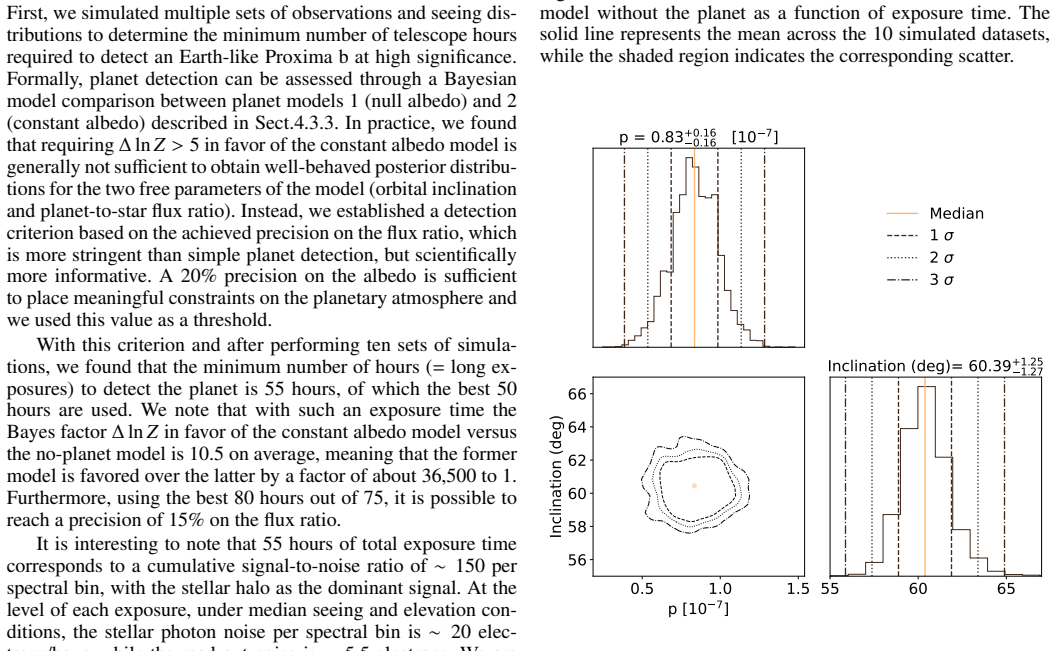
- [Sec. 4.3.1; Sec. 5.2.1] The 20% albedo 'precision' reported in Sec. 5.2.1 is statistical precision only. The same section states that the mean flux ratio is underestimated by ~20% because the third coupling-function ratio rho^p_i(r)/rho^s_i(r_off) is set to 1 in the model (Sec. 4.3.1). Thus the demonstrated capability is a 20%-wide posterior centered ~20% below the true value, which does not by itself establish 20%-accurate albedo characterization. Please provide a combined statistical+systematic error budget, or rephrase the claim as '20% statistical precision before calibration of the planet-position coupling ratio.'
minor comments (3)
- [Sec. 5.1] The sentence 'using the best 80 hours out of 75' appears to be a typo; presumably it should read 'best 75 out of 80' or similar. Please correct.
- [Sec. 4.2, Eq. (8)] The notation <F1/F2>_o is used before the weighted average is defined in the preceding paragraph; consider adding a brief definition at the point of first use to help the reader.
- [Sec. 2.1.1] The statement that the IFU projects 'approximately 37 milliarcseconds between the centers of adjacent spaxels' is ambiguous: it would be clearer to specify the spaxel pitch and the lenslet size separately, since the coupling maps in Fig. 8 are plotted in milliarcseconds.
Circularity Check
The 55-h planet detection is an independent injection-recovery result, but the 85-h O2/H2O molecular detection is an in-sample matched filter: the 'full albedo spectrum' model is the exact spectrum used to generate the synthetic data, so the molecular detection is built in by construction.
specific steps
-
fitted input called prediction
[Abstract; Sect. 4.3.3 'Full albedo spectrum'; Sect. 5.2.3 and Fig. 19; Sect. 7.1]
"we only consider the exact same albedo spectrum that was used to generate the simulated spectra ... The actual parameter space of the model has been reduced to two dimensions because we have access to the 'true' planetary albedo spectrum (i.e., the one we used to build our synthetic observations)."
The full albedo model is given the identical molecular absorption spectrum that was used to generate the simulated observations, with only a global scaling and inclination left free. The 80-85 h 'molecular signatures distinguishable' claim (Fig. 19) therefore measures the evidence for the injected template, not an independent detection of O2 or H2O. Because the model and the data generator share the same molecular absorption features, the Bayes-factor growth is forced by construction. The abstract's statement that 'molecular absorption by O2 and H2O can be detected in about 85 hours' is an in-sample matched-filter result. This is confirmed by Sec. 5.2.4, where the independent single-layer HITRAN model detects O2 at 100 h but yields 'close to zero' preference for H2O, contradicting the abst
full rationale
The paper's central 55-h detection claim is not circular: it is obtained with a constant-albedo model (Eq. 10) that does not use the injected spectrum's molecular structure, and it is validated against the no-planet model with a Bayes-factor threshold plus a 20% albedo-precision criterion. The orbital inclination recovery and the spin-axis constraint method are also independent, self-contained simulations. However, the second headline result—85 h for O2 and H2O molecular detection—does reduce by construction. The 'full albedo spectrum' model in Sect. 4.3.3 explicitly adopts the exact GCM/PICASO spectrum used to make the synthetic data, with only a free scaling. Consequently, the 80-85 h molecular detection in Fig. 19 is a matched filter on the truth, not a blind or physically motivated molecular detection. The paper is transparent about this in Sects. 5.2.3 and 7.1, but the abstract overstates it, and the independent HITRAN molecular model in Sec. 5.2.4 finds no H2O preference even at 100 h, making the abstract's H2O claim internally inconsistent. Other cited inputs, notably the IFU coupling functions from Blind et al. (2024), are external end-to-end instrument simulations and do not constitute circularity. Overall: one central sub-claim reduces to its input by construction, while the primary planet-detection claim remains independent, giving partial circularity.
Axiom & Free-Parameter Ledger
free parameters (9)
- Planet-to-star flux ratio p (constant albedo model) =
p = 0.83 +/- 0.16 x 1e-7 for the 55-hour example; true injected value about 1e-7, with mean underestimated by about 20%
- Orbital inclination i =
60.39 +/- 1.27 deg in example posterior; true value 60 deg
- Chromatic albedo bin values p_1..p_n =
n = 2, 3, 5, 10 bins over 620-840 nm; 5-parameter fit shown in Fig. 18
- Full albedo scaling factor =
Not quoted separately; multiplicative factor on the injected GCM/PICASO albedo spectrum
- Molecular column density N =
O2 model: N = 7.62 +1.70/-3.09 x 1e26 mol/cm2; H2O model: N = 3.58 +6.64/-2.54 x 1e21 mol/cm2
- Molecular pressure P =
O2 P = 2.38 +0.90/-0.67 bar; H2O P = 0.84 +0.74/-0.64 bar; temperature fixed at 250 K
- Third coupling function ratio rho_p_i(r)/rho_s_i(roff) =
Assumed 1.0; true simulation value about 0.86
- Spin-axis sine amplitude A =
A = 2.21 +/- 0.10 m/s for one MCMC example
- Stellar spin axis orientation theta_s =
Recovered within +/-5.4 deg of true value 0 across 10 simulations
axioms (8)
- domain assumption Proxima b orbital elements from Mascareno et al. (2025) are correct, with eccentricity fixed to 0.
- domain assumption The PHOENIX synthetic spectrum accurately represents Proxima's stellar spectrum; stellar activity and flares are neglected.
- domain assumption The GCM/PICASO Earth-like atmosphere (1 bar N2-O2, 400 ppm CO2, water surface, self-consistent clouds) produces a realistic reflected planet spectrum.
- domain assumption The RISTRETTO AO plus coronagraph coupling functions from Blind et al. (2024) predict on-sky performance.
- domain assumption The stellar spin axis is aligned with the Proxima b orbital plane (small obliquity).
- domain assumption The planet reflected spectrum is fixed at a 90-degree orbital phase angle for all epochs; phase function variations are ignored.
- ad hoc to paper The full albedo model uses exactly the injected albedo spectrum, without exploring the true GCM parameter space.
- ad hoc to paper The best 90-95% of exposures are selected a posteriori, and the 55-hour estimate uses the best 50 of 55 one-hour exposures.
Cite this review
Pith. "Pith review of Simulating RISTRETTO: Proxima b detectability in reflected light." pith.science (2026). https://pith.science/paper/NVKM6AJN
@misc{pith2026250907644,
  author       = {Pith},
  title        = {Pith review of: Simulating RISTRETTO: Proxima b detectability in reflected light},
  year         = {2026},
  howpublished = {\url{https://pith.science/paper/NVKM6AJN}},
  note         = {Machine review of arXiv:2509.07644}
}
abstract
The characterization of exoplanet atmospheres is one of the key topics in modern astrophysics. To date, transmission spectroscopy has been the primary method used, but upcoming instruments will lay the foundation for advancing reflected-light spectroscopy. The main challenge in this area of research is the high contrast ratio between the planet and its star. RISTRETTO, a high-resolution integral-field spectrograph designed for ESO's VLT, aims to address these limitations through a combination of extreme AO, coronagraphy, and high-resolution spectroscopy. The goal of this paper is to demonstrate the detectability of the temperate rocky planet Proxima b with RISTRETTO, using realistic end-to-end simulations and a specifically developed data analysis methodology. We created high-resolution star and planet spectra, selecting realistic observational epochs and incorporating the predicted performance of the AO and coronagraphic systems. We implemented noise and spectrograph effects through the Pyechelle spectrograph simulator. We then applied a new methodology to isolate the signal of the planet from the stellar one and proceeded to fit several planetary models in order of increasing complexity. We also introduced a method to determine the sky orientation of the stellar spin axis, which constrains the orientation of the planetary orbit for aligned systems. Assuming an Earth-like atmosphere, our results show that RISTRETTO can detect Proxima b in reflected light in about 55 hours of observing time, offering the ability to characterize the planet orbital inclination, true mass, and broadband albedo. In addition, molecular absorption by O$_2$ and H$_2$O can be detected in about 85 hours of observations. These findings highlight the potential of RISTRETTO to significantly advance the field of exoplanetary science by enabling reflected-light spectroscopy of a sample of nearby exoplanets.
Figures




Forward citations
Cited by 1 Pith paper
-
Magnetic field strengths of hot giant exoplanets consistent with Solar System values
Wind speed measurements in seven ultra-hot Jupiters decrease with temperature, consistent with magnetic drag and implying magnetic field strengths of a few gauss.
Reference graph
Works this paper leans on
-
[1]
2024, A&A, 689, A245 Anglada-Escudé, G., Amado, P
Alei, E., Quanz, S., Konrad, B., et al. 2024, A&A, 689, A245 Anglada-Escudé, G., Amado, P. J., Barnes, J., et al. 2016, nature, 536, 437
work page 2024
-
[2]
D., Ruane, G., Jovanovic, N., et al
Baker, A. D., Ruane, G., Jovanovic, N., et al. 2024, in Ground-based and Air- borne Instrumentation for Astronomy X, V ol. 13096, SPIE, 130961G
work page 2024
-
[3]
Batalha, N. E., Marley, M. S., Lewis, N. K., & Fortney, J. J. 2019, ApJ, 878, 70
work page 2019
-
[4]
Blind, N., Restori, N., . Chazelas, B., et al. 2025, arXiv e-prints, arXiv:2503.18538
-
[5]
2024, in Adaptive Optics Systems IX, V ol
Blind, N., Shinde, M., Dinis, I., et al. 2024, in Adaptive Optics Systems IX, V ol. 13097, SPIE, 1622–1634
work page 2024
-
[6]
Bonfils, X., Delfosse, X., Udry, S., et al. 2013, A&A, 549, A109
work page 2013
-
[7]
J., Koch, D., Basri, G., et al
Borucki, W. J., Koch, D., Basri, G., et al. 2010, Science, 327, 977
2010
- [8]
-
[9]
Bourrier, V ., Delisle, J.-B., Lovis, C., et al. 2024, A&A, 691, A113
work page 2024
-
[10]
S., V on Braun, K., Van Belle, G., et al
Boyajian, T. S., V on Braun, K., Van Belle, G., et al. 2012, ApJ, 757, 112
work page 2012
-
[11]
2016, Statistics and Computing, 26, 383
Buchner, J. 2016, Statistics and Computing, 26, 383
2016
-
[12]
2019, PASP, 131, 108005
Buchner, J. 2019, PASP, 131, 108005
2019
-
[13]
2021, The Journal of Open Source Software, 6, 3001
Buchner, J. 2021, The Journal of Open Source Software, 6, 3001
2021
-
[14]
J., et al
Cadieux, C., Doyon, R., MacDonald, R. J., et al. 2024, ApJL, 970, L2
2024
-
[15]
2024, in Ground-based and Airborne Instrumentation for Astronomy X, V ol
Chazelas, B., Lovis, C., Blind, N., et al. 2024, in Ground-based and Airborne Instrumentation for Astronomy X, V ol. 13096, SPIE, 2201–2209
work page 2024
-
[16]
Currie, M. H. & Meadows, V . S. 2025, , 6, 96
work page 2025
-
[17]
Damiano, M. & Hu, R. 2021, AJ, 162, 200
work page 2021
-
[18]
Dressing, C. D. & Charbonneau, D. 2013, ApJ, 767, 95
work page 2013
-
[19]
2023 European Southern Observatory
Ducrot, E., Lagage, P.-O., Min, M., et al. 2023 European Southern Observatory. 2024
work page 2023
- [20]
-
[21]
2024, in Space Telescopes and Instru- mentation 2024: Optical, Infrared, and Millimeter Wave, V ol
Feinberg, L., Ziemer, J., Ansdell, M., et al. 2024, in Space Telescopes and Instru- mentation 2024: Optical, Infrared, and Millimeter Wave, V ol. 13092, SPIE, 511–522
work page 2024
- [22]
-
[23]
Fischer, D. A. 2021, in ExoFrontiers: Big questions in exoplanetary science (IOP Publishing Bristol, UK), 4–1
work page 2021
-
[24]
W., Lang, D., & Goodman, J
Foreman-Mackey, D., Hogg, D. W., Lang, D., & Goodman, J. 2013, PASP, 125, 306
2013
-
[25]
Foreman-Mackey, D., Morton, T. D., Hogg, D. W., Agol, E., & Schölkopf, B. 2016, AJ, 152, 206 Gaia Collaboration, Brown, A. G. A., Vallenari, A., et al. 2021, A&A, 649, A1
work page 2016
-
[26]
Gaidos, E., Mann, A., Kraus, A., & Ireland, M. 2016, MNRAS, 457, 2877
work page 2016
-
[27]
Gialluca, M. T., Robinson, T. D., Rugheimer, S., & Wunderlich, F. 2021, PASP, 133, 054401
work page 2021
-
[28]
Gordon, I. E., Rothman, L. S., Hargreaves, e. R., et al. 2022, Journal of quanti- tative spectroscopy and radiative transfer, 277, 107949
work page 2022
-
[29]
2024, in Adaptive Optics Systems
Guyon, O., Vievard, S., Lallement, M., et al. 2024, in Adaptive Optics Systems
work page 2024
-
[30]
Hatzes, A. P. 2016, Methods of Detecting Exoplanets: 1st Advanced School on Exoplanetary Science, 3
work page 2016
-
[31]
Hoeijmakers, H., Snellen, I., & Van Terwisga, S. 2018, A&A, 610, A47
work page 2018
-
[32]
Horak, H. G. 1950, PhD thesis, The University of Chicago
work page 1950
-
[33]
2013, A&A, 553, A6
Husser, T.-O., Wende-von Berg, S., Dreizler, S., et al. 2013, A&A, 553, A6
2013
- [34]
- [35]
-
[36]
Kasper, M., Cerpa Urra, N., Pathak, P., et al. 2021, The Messenger, 182, 38
work page 2021
-
[37]
V ., Gordon, I., Rothman, L., et al
Kochanov, R. V ., Gordon, I., Rothman, L., et al. 2016, Journal of Quantitative Spectroscopy and Radiative Transfer, 177, 15
work page 2016
-
[38]
Landman, R., Stolker, T., Snellen, I., et al. 2024, A&A, 682, A48
work page 2024
-
[39]
Larkin, J. E., Moore, A. M., Wright, S. A., et al. 2016, in Ground-based and Airborne Instrumentation for Astronomy VI, V ol. 9908, SPIE, 582–594 Lecavelier Des Etangs, A., Pont, F., Vidal-Madjar, A., & Sing, D. 2008, A&A, 481, L83
work page 2016
- [40]
-
[41]
Lewis, N. K., Showman, A. P., Fortney, J. J., Knutson, H. A., & Marley, M. S. 2014, ApJ, 795, 150
work page 2014
-
[42]
2023, ApJL, 955, L22
Lim, O., Benneke, B., Doyon, R., et al. 2023, ApJL, 955, L22
2023
-
[43]
2024, in Ground-based and Airborne Instrumentation for Astronomy X, V ol
Lovis, C., Blind, N., Chazelas, B., et al. 2024, in Ground-based and Airborne Instrumentation for Astronomy X, V ol. 13096, SPIE, 412–417
work page 2024
- [44]
- [45]
-
[46]
Mann, A. W., Feiden, G. A., Gaidos, E., Boyajian, T., & V on Braun, K. 2015, ApJ, 804, 64
work page 2015
-
[47]
2022, in Ground-based and Air- borne Instrumentation for Astronomy IX, V ol
Marconi, A., Abreu, M., Adibekyan, V ., et al. 2022, in Ground-based and Air- borne Instrumentation for Astronomy IX, V ol. 12184, SPIE, 720–735
work page 2022
-
[48]
2015, A&A, 576, A134 Mascareño, A
Martins, J., Santos, N., Figueira, P., et al. 2015, A&A, 576, A134 Mascareño, A. S., Faria, J., Figueira, P., et al. 2020, A&A, 639, A77 Mascareño, A. S. et al. 2025, A&A, accepted for publication
work page 2015
-
[49]
& Queloz, D
Mayor, M. & Queloz, D. 1995, Nature, 378, 355
1995
-
[50]
Mulders, G. D., Pascucci, I., & Apai, D. 2015, ApJ, 814, 130
work page 2015
-
[51]
2012, A&A, 543, A92
Noll, S., Kausch, W., Barden, M., et al. 2012, A&A, 543, A92
2012
-
[52]
2018, in Ground-based and Airborne Instrumentation for Astronomy VII, V ol
Packham, C., Honda, M., Chun, M., et al. 2018, in Ground-based and Airborne Instrumentation for Astronomy VII, V ol. 10702, SPIE, 3118–3129
work page 2018
-
[53]
2025, Experimental Astronomy, 59, 1
Palle, E., Biazzo, K., Bolmont, E., et al. 2025, Experimental Astronomy, 59, 1
work page 2025
-
[54]
Parc, L., Bouchy, F., Venturini, J., Dorn, C., & Helled, R. 2024, A&A, 688, A59
work page 2024
-
[55]
2021, in ExoFrontiers: Big questions in exoplanetary science (IOP Publishing Bristol, UK), 3–1
Pollacco, D., Batalha, N., Deleuil, M., & Ricker, G. 2021, in ExoFrontiers: Big questions in exoplanetary science (IOP Publishing Bristol, UK), 3–1
work page 2021
-
[56]
V ., Apai, D., & Giampapa, M
Rackham, B. V ., Apai, D., & Giampapa, M. S. 2018, ApJ, 853, 122
2018
-
[57]
Restori, N., Blind, N., Kühn, J., et al. 2024, in Advances in Optical and Mechan- ical Technologies for Telescopes and Instrumentation VI, V ol. 13100, SPIE, 853–863
work page 2024
-
[58]
Ribas, I., Gregg, M. D., Boyajian, T. S., & Bolmont, E. 2017, A&A, 603, A58
work page 2017
-
[59]
1981, in Progress in optics, V ol
Roddier, F. 1981, in Progress in optics, V ol. 19 (Elsevier), 281–376
work page 1981
-
[60]
M., et al
Ruffio, J.-B., Macintosh, B., Konopacky, Q. M., et al. 2019, AJ, 158, 200
2019
-
[61]
& Sasselov, D
Seager, S. & Sasselov, D. D. 2000, ApJ, 537, 916
2000
- [62]
-
[63]
2006, Bayesian Analysis, 1
Skilling, J. 2006, Bayesian Analysis, 1
2006
-
[64]
Snellen, I., Albrecht, S., De Mooij, E., & Le Poole, R. 2008, A&A, 487, 357
work page 2008
- [65]
-
[66]
Snellen, I. A. 2025, ARA&A, 63
work page 2025
-
[67]
Sparks, W. B. & Ford, H. C. 2002, ApJ, 578, 543 Stürmer, J., Seifahrt, A., Robertson, Z., Schwab, C., & Bean, J. L. 2018, PASP, 131, 024502
work page 2002
-
[68]
2008, Contemporary Physics, 49, 71
Trotta, R. 2008, Contemporary Physics, 49, 71
2008
-
[69]
Turbet, M., Leconte, J., Selsis, F., et al. 2016, A&A, 596, A112
work page 2016
-
[70]
Vaughan, S. R., Birkby, J. L., Thatte, N., et al. 2024, MNRAS, 528, 3509
work page 2024
-
[71]
Wang, J., Mawet, D., Ruane, G., Hu, R., & Benneke, B. 2017, AJ, 153, 183
work page 2017
-
[72]
Winn, J. N. & Fabrycky, D. C. 2015, ARA&A, 53, 409
2015
-
[73]
2023, ZEMAX Optical Design Software, accessed on December 18, 2023
Zemax, LLC. 2023, ZEMAX Optical Design Software, accessed on December 18, 2023
work page 2023
-
[74]
2023, Nature, 620, 746 Article number, page 17 of 18 A&A proofs: manuscript no
Zieba, S., Kreidberg, L., Ducrot, E., et al. 2023, Nature, 620, 746 Article number, page 17 of 18 A&A proofs: manuscript no. output Appendix A: Barycentric radial velocities during the observational epochs Feb Mar Apr May Jun Jul 15 10 5 0 5 10 15 20 Barycentric RV (km/s) Fig. A.1: Barycentric correction during the observational epochs Appendix B: Star sp...
work page 2023
This paper was first reviewed by deepseek-v4-flash on August 4, 2026.
discussion (0)
Sign in with ORCID, Apple, or X to comment. Anyone can read and Pith papers without signing in.