Pith. sign in

REVIEW 3 major objections 6 minor 16 references

This thesis proves that error feedback with contractive compressors converges in O((L + L_AM ξ(α))/ε) rounds, replacing the quadratic mean of client smoothness constants with their arithmetic mean.

Reviewed by Pith at T0; open to challenge. T0 means a machine referee read the full paper against a public rubric. the ladder, T0–T4 →

T0 review · deepseek-v4-flash

2026-08-04 21:14 UTC pith:5YREGSGB

load-bearing objection A solid, well-organized PhD thesis that consolidates the author's previously published work; the EF21-W chapter is mathematically sound and the engineering chapters are substantial, but the empirical speedup claims and reliance on known per-client smoothness constants deserve scrutiny. the 3 major comments →

arxiv 2509.08120 v1 pith:5YREGSGB submitted 2025-09-09 cs.LG math.OC

Optimization Methods and Software for Federated Learning

classification cs.LG math.OC MSC 68W4090C26
keywords federated learningerror feedbackEF21-Wcommunication compressionsmoothness heterogeneitynonconvex optimizationdistributed trainingFedNL
verification ladder T0 review T1 audit T2 compute T3 formal T4 reserved

The pith

A machine-rendered reading of the paper's core claim, the machinery that carries it, and where it could break.

The thesis tackles five challenges in federated learning—heterogeneous data, heterogeneous devices, communication bottlenecks, privacy, and the gap between theory and usable software. Its central theoretical result is that error feedback with contractive compressors (EF21) can be analyzed with the arithmetic mean of per-client smoothness constants instead of the quadratic mean, so heterogeneous smoothness is less costly than previously proven. The mechanism is a smoothness-weighted variant, EF21-W, and a weighted analysis of vanilla EF21; both admit step sizes up to 1/(L + L_AM ξ(α)) and therefore communication complexity O((L + L_AM ξ(α))/ε). The same weighting transfers to stochastic-gradient and partial-participation variants and to Polyak-Łojasiewicz and rare-features settings. Around this theory, the thesis builds practical software: a federated simulation environment, a fast FedNL implementation, and a high-speed CPU backpropagation framework.

Core claim

For minimizing f(x)=1/n Σ f_i(x) under L-smoothness of f and L_i-smoothness of each f_i, the paper proves that EF21—the best-known error-feedback method for contractive compressors—needs only T = O((L + L_AM ξ(α))/ε) iterations to reach E‖∇f(x̂)‖² ≤ ε, where L_AM = (1/n)Σ L_i and ξ(α) depends only on the compressor's contraction parameter. Previously the best bound had L_QM = sqrt((1/n)Σ L_i²) in place of L_AM. The improvement is obtained three ways: by cloning each client N_i times with frequencies ⌈L_i/L_AM⌉ (a √2-approximate optimal scheme), by the weighted algorithm EF21-W with weights w_i = L_i/Σ_j L_j, and by a weighted analysis of unweighted EF21. The proof introduces a weighted gradi

What carries the argument

The carrying identity is w_i = L_i / Σ_j L_j: with these weights, EF21-W's server update is x^{t+1} = x^t − γ Σ_i w_i g_i^t, and the weighted distortion G^t = Σ_i w_i ‖g_i^t − ∇f_i(x^t)/(n w_i)‖² obeys a contraction whose residual coefficient is L_AM² rather than L_QM². The same weights inserted into the proof for vanilla EF21, via Jensen's inequality on the distortion, deliver the same rate without modifying the algorithm. Client cloning is the discovery route: replicating client i to N_i copies with rescaled functions reduces the quadratic mean to the arithmetic mean; integer cloning frequencies ⌈L_i/L_AM⌉ are a √2-approximation and need at most 2n total clients.

Load-bearing premise

The step size and the weights in EF21-W require exact knowledge of every client's smoothness constant L_i; if these constants are estimated or tuned imperfectly, the advertised step size bound and convergence complexity no longer hold.

What would settle it

Take a non-convex problem with n=1000 clients where one client has smoothness 100 times the others, run EF21 and EF21-W with the Top1 compressor and the theoretical steps from Theorem 8 versus the old bound, and record rounds to reach E‖∇f‖² ≤ ε. If EF21-W's rounds do not follow (L + L_AM ξ(α))/ε, or if perturbing the claimed optimal weights w_i by 10% drives the method to diverge at the theoretical step size, the central claim fails.

Watch this falsifier. Get emailed when new claim-graph text bears on it.

If this is right

  • Communication complexity of EF21-style methods with contractive compressors becomes O((L + L_AM ξ(α))/ε), so heterogeneous smoothness between clients is less harmful than the earlier L_QM bound suggested.
  • EF21-W permits theoretical step size γ ≤ 1/(L + L_AM ξ(α)), which is larger than the L_QM-based step whenever L_QM > L_AM, yielding fewer communication rounds in the experiments.
  • The weighted analysis extends to EF21-SGD, EF21-PP, PL functions, and the rare-features regime, so the L_AM improvement is not limited to full-gradient full-participation EF21.
  • Cloning shows that adding rescaling clients can improve rates: at most 2n virtual clients suffice to get within √2 of the optimal cloning objective.
  • Experiments on non-convex logistic regression and synthetic linear problems show the largest gains when L_var = L_QM² − L_AM² is large.

Where Pith is reading between the lines

These are editorial extensions of the paper, not claims the author makes directly.

  • If exact L_i are unavailable, the theory suggests an online estimator for w_i could still capture much of the benefit; a testable extension is to replace L_i with running estimates of local gradient Lipschitz constants and measure whether the step-size validity holds.
  • The equivalence between cloning and weighting hints that the L_AM rate may extend to other biased compressors (RankK, natural compression) and to decentralized topologies where each node's 'clones' are weighted aggregations.
  • The same weighted-distortion technique could sharpen rates for second-order FL methods like FedNL by replacing worst-case client smoothness with an arithmetic-mean dependence.

Editorial analysis

A structured set of objections, weighed in public.

Desk editor's note, referee report, simulated authors' rebuttal, and a circularity audit.

Referee Report

3 major / 6 minor

Summary. The dissertation addresses five challenges in Federated Learning (FL) across seven chapters, each a previously published paper. The central theoretical contribution is in Chapter 3, where the author replaces the quadratic mean (L_QM) of client smoothness constants in the EF21 error-feedback method with the arithmetic mean (L_AM), yielding the communication complexity T = O((L + L_AM * xi(alpha))/epsilon) for non-convex smooth objectives. This is achieved through three routes: client cloning, a new weighted algorithm EF21-W (Algorithm 3), and a weighted analysis of the original EF21. The other chapters present FL_PyTorch, a simulation framework; DCGD/PermK/AES, a classical-cryptography approach to private FL; refined PAGE analysis; compressed personalized L2GD; a high-performance FedNL implementation; and BurTorch, a low-latency backpropagation engine. The thesis emphasizes the interplay between theory, systems, and practical implementation, with each chapter containing its own reproducibility appendix.

Significance. If the Chapter 3 result is correct, it is a genuine improvement over the best-known communication complexity for algorithms using contractive compressors, replacing a potentially much larger quadratic-mean constant with the arithmetic mean. The proofs are self-contained and the derivation of the weights w_i = L_i / sum_j L_j is structurally sound. The systems chapters provide substantial engineering contributions, and the thesis explicitly ships reproducibility statements and code links for several chapters. However, the practical applicability claims rest on assumptions that are not stress-tested: exact knowledge of per-client smoothness constants in EF21-W, no sensitivity analysis in the experiments, and performance claims (x1000 speedup, x3500 memory reduction) that are not fully verifiable from the manuscript alone. The significance is therefore real but tempered by the gap between the stated theoretical conditions and the claimed practical readiness.

major comments (3)
  1. [Chapter 3, Theorem 8 / Algorithm 3] The central practical claim of Section 3.3 relies on exact knowledge of each L_i to set w_i = L_i / sum_j L_j and gamma <= 1/(L + L_AM * xi(alpha)). The proof in Appendix C3.2 requires the inequality gamma^2 * beta * L_AM^2 / theta + L * gamma <= 1. If L_AM is underestimated, the implemented gamma can violate this bound and the contraction argument collapses. Overestimating preserves correctness but degrades the rate. The experiments report 'theoretical step sizes' but do not state how L_i were obtained or how sensitive the method is to misspecification. This is load-bearing for the thesis's applicability claims, and it conflicts with the thesis's own principle stated in Section 1.2.5 that estimation costs should be accounted for in final evaluation. I recommend adding a sensitivity analysis and discussing practical estimation of L_i.
  2. [Chapter 3, Theorem 9] The improved theory for the original EF21 also assumes knowledge of L_i to set the step size via L_AM and the analysis uses weights w_i = L_i / sum_j L_j in the Lyapunov argument (Appendix D3). The text (Section 3.2.4) suggests that EF21 inherits the L_AM rate automatically for positively homogeneous compressors, but in practice the step size still requires exact smoothness constants. The manuscript does not discuss how practitioners should obtain these constants in federated settings, nor does it analyze the robustness of Theorem 9 to inexact L_i. This is a gap between the stated theoretical improvement and the claimed practical impact.
  3. [Chapters 7 and 8] The performance claims - x1000 wall-clock improvement for FedNL (Section 7.5) and up to x2000/x3500 runtime/memory improvements for BurTorch (Chapter 8, Table 8.1) - are central to the software contributions. The manuscript provides detailed optimization narratives and reproducibility appendices, but the full experimental code is not included in the arXiv submission, and the baselines are compared against a specific reference implementation and specific framework versions. This makes independent verification difficult. Given that the thesis explicitly positions practical implementation as a key contribution, the lack of a complete, self-contained benchmark suite or measurement scripts in the manuscript is a significant gap.
minor comments (6)
  1. [Section 3.3] The phrase 'partial partial participation' appears twice (Figures 3.2 caption and text). The intended expression is likely 'partial participation' or 'random client participation'.
  2. [Table 7.4] The title contains a typo: 'Improvemens' should be 'Improvements'.
  3. [Appendix A3.4] The heading '2-Suboptimal but simple step size rule' is unclear; the '2-' prefix is not explained. Presumably it means the step size is within a factor of 2 of optimal, but this should be stated.
  4. [Appendix E3.3, Theorem 13] The condition for choosing s and mu uses both 'mu' and 'nu' with inconsistent notation: the algorithm defines nu, but the condition states (1+s)(1+mu)<1/(1-alpha). This should be unified.
  5. [Appendix E3.2, Lemma 10 proof] Several intermediate lines contain garbled or duplicated symbols (e.g., '\\|\\nabla f_i(x^{t+1}) -' followed immediately by '\\|\\nabla f_i(x^t)\\|^2\\|'). These appear to be formatting errors from the LaTeX conversion; please correct.
  6. [Section 1.5.3, Definition 6] The phrase 'conically bounded variance' is used but not defined. If this is standard, a reference or definition is needed.

Circularity Check

0 steps flagged

No significant circularity; EF21-W's L_AM rate is a self-contained theorem from stated smoothness assumptions, not a fitted or self-citational reduction.

full rationale

The strongest claimed contribution, replacing L_QM by L_AM in EF21's communication complexity, is derived independently in Chapter 3. The proof of Theorem 8 (Appendix C3) starts from Assumptions 1-3 and the contractive-compressor definition, constructs the Lyapunov function G^t = \sum_i w_i ||g_i^t - (1/(n w_i))\nabla f_i(x^t)||^2, and obtains the coefficient L_AM^2 from the algebraic identity \sum_i L_i^2/w_i = n^2 L_AM^2 after setting w_i = L_i / \sum_j L_j (Lemma 7, Eq. 3.30). This is a direct calculation, not a parameter fitted to data or a renamed known result. Theorem 9 similarly re-weights the analysis of the original EF21 and proves the same identity (Appendix D3, Lemma 8). The step-size condition and the resulting T = O((L + L_AM \xi(\alpha))/\varepsilon) are consequences of the Lyapunov inequality, not assumptions equivalent to the conclusion. The paper's reliance on exact knowledge of L_i is a genuine practical limitation, and the thesis itself flags the estimation cost in Section 1.2.5, but this is a conditional guarantee, not circularity. Citations to Richtárik et al. (2021a) supply standard lemmas (descent inequality, Young's inequality, a scalar bound) that are elementary and not the target result; they do not carry the EF21-W conclusion. The experimental sections use theoretical step sizes and do not fit convergence rates to measured data. I therefore find no circular step that reduces a prediction to its inputs.

Axiom & Free-Parameter Ledger

1 free parameters · 5 axioms · 0 invented entities

The central theoretical results rest on standard smoothness, compression, and boundedness assumptions; no new axioms beyond the cited literature are introduced. The free parameter listed is purely experimental.

free parameters (1)
  • Regularization coefficient lambda in EF21-W experiments = 0.001 or 1000 (chosen by hand)
    Set per experiment for numerical stability; not part of the algorithm's theoretical guarantee.
axioms (5)
  • domain assumption f and f_i are L- and L_i-smooth (Assumptions 1 and 2, Chapter 3)
    Standard smoothness conditions used throughout the thesis for convergence analysis.
  • domain assumption f is lower bounded (Assumption 3, Chapter 3)
    Necessary for meaningful minimization.
  • standard math Contractive compression operators satisfy E||C(x)-x||^2 <= (1-alpha)||x||^2 (Definition 6, Chapter 3)
    Standard definition of biased compressors.
  • domain assumption Polyak-Lojasiewicz condition (Assumption 4, Chapter 3)
    Used to derive linear convergence results in some theorems.
  • domain assumption Stochastic gradient estimator bound (Assumption 5, Chapter 3 appendix)
    Used in the EF21-W-SGD analysis, a general non-convex stochastic gradient condition.

pith-pipeline@v1.3.0-alltime-deepseek · 169 in / 9816 out tokens · 137550 ms · 2026-08-04T21:14:35.054982+00:00 · methodology

0 comments
read the original abstract

Federated Learning (FL) is a novel, multidisciplinary Machine Learning paradigm where multiple clients, such as mobile devices, collaborate to solve machine learning problems. Initially introduced in Kone{\v{c}}n{\'y} et al. (2016a,b); McMahan et al. (2017), FL has gained further attention through its inclusion in the National AI Research and Development Strategic Plan (2023 Update) of the United States (Science and on Artificial Intelligence, 2023). The FL training process is inherently decentralized and often takes place in less controlled settings compared to data centers, posing unique challenges distinct from those in fully controlled environments. In this thesis, we identify five key challenges in Federated Learning and propose novel approaches to address them. These challenges arise from the heterogeneity of data and devices, communication issues, and privacy concerns for clients in FL training. Moreover, even well-established theoretical advances in FL require diverse forms of practical implementation to enhance their real-world applicability. Our contributions advance FL algorithms and systems, bridging theoretical advancements and practical implementations. More broadly, our work serves as a guide for researchers navigating the complexities of translating theoretical methods into efficient real-world implementations and software. Additionally, it offers insights into the reverse process of adapting practical implementation aspects back into theoretical algorithm design. This reverse process is particularly intriguing, as the practical perspective compels us to examine the underlying mechanics and flexibilities of algorithms more deeply, often uncovering new dimensions of the algorithms under study.

Figures

Figures reproduced from arXiv: 2509.08120 by Konstantin Burlachenko.
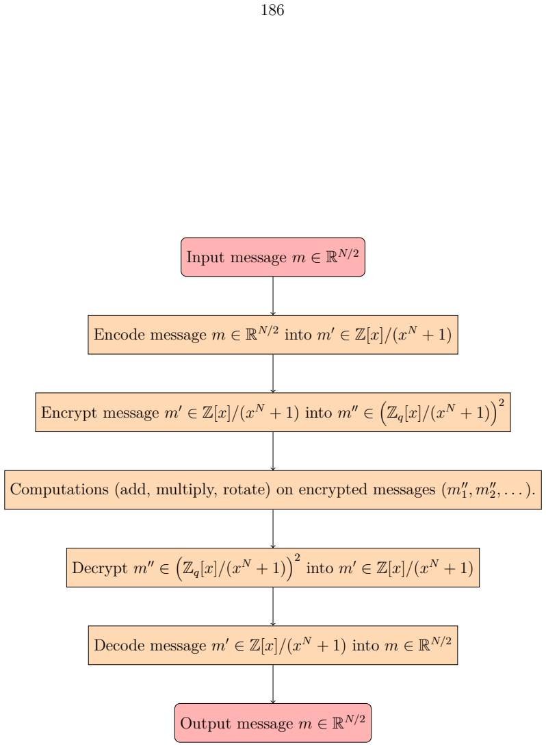
Figure 1.1
Figure 1.1. Figure 1.1: The lifecycle of a Federated Learning training in the cross-device [PITH_FULL_IMAGE:figures/full_fig_p029_1_1.png] view at source ↗
Figure 1.2
Figure 1.2. Figure 1.2: The interconnections between various aspects of Federated Learning [PITH_FULL_IMAGE:figures/full_fig_p036_1_2.png] view at source ↗
Figure 2.1
Figure 2.1. Figure 2.1: Graphical User Interface (GUI) of the FL_PyTorch simulator [PITH_FULL_IMAGE:figures/full_fig_p049_2_1.png] view at source ↗
Figure 2.2
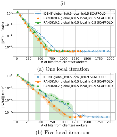
Figure 2.2. Figure 2.2: Function gradient diminishing for 1 and 5 local iterations of [PITH_FULL_IMAGE:figures/full_fig_p051_2_2.png] view at source ↗
Figure 2.3
Figure 2.3. Figure 2.3: Experiments with MARINA and DIANA algorithms with making local steps for quadratic minimization. Mean and variance have been estimated across 10 realizations. 0 25 50 75 100 125 150 175 200 Rounds 1.2 × 10 0 1.4 × 10 0 1.6 × 10 0 1.8 × 10 0 2 × 10 0 2.2 × 10 0 2.4 × 10 0 2.6 × 10 0 || F ( x )|| ( t r ain ) BERNULLI:0.1 INTERNAL_SGD:FULL-GRADIENT MARINA BERNULLI:0.1 INTERNAL_SGD:SGD-NICE,TAU:10% MARINA BE… view at source ↗
Figure 2.4
Figure 2.4. Figure 2.4: Experiments with MARINA and DIANA algorithms for training ResNet￾18 on CIFAR-10 dataset. a significant decrease in performance This experiment was carried out on a synthetically generated quadratic mini￾mization Problem (2.3). We set the dimensionality of the problem to be 20. Both features 𝑎𝑖 ’s and responses 𝑏𝑖 are generated using a uniform distribution on the interval [0, 1]. After this step, we updat… view at source ↗
Figure 2.5
Figure 2.5. Figure 2.5: A single worker thread structure and its role in a thread pool. [PITH_FULL_IMAGE:figures/full_fig_p058_2_5.png] view at source ↗
Figure 2.6
Figure 2.6. Figure 2.6: FL_PyTorch execution context for a single experiment. The GUI can handle several experiments at the same time [PITH_FULL_IMAGE:figures/full_fig_p058_2_6.png] view at source ↗
Figure 2.7
Figure 2.7. Figure 2.7: Communication between different threads during Algorithm [PITH_FULL_IMAGE:figures/full_fig_p059_2_7.png] view at source ↗
Figure 2.8
Figure 2.8. Figure 2.8: NVIDIA compute ecosystem and the place of [PITH_FULL_IMAGE:figures/full_fig_p061_2_8.png] view at source ↗
Figure 3.1
Figure 3.1. Figure 3.1: Comparison of EF21 versus our new EF21-W with the Top1 compressor on the non-convex logistic regression problem. The number of clients 𝑛 is 1,000. The step size for EF21 is set according to (Richtárik et al., 2021a), and the step size for EF21-W is set according to Theorem 8. The coefficient 𝜆 for (b)– (f) is set to 0.001, and for (a) is set to 1,000 for numerical stability. We let 𝐿var def = 𝐿 2 QM − 𝐿 … view at source ↗
Figure 3.2
Figure 3.2. Figure 3.2: Comparison of EF21-W with partial partial participation (EF21-W-PP) or stochastic gradients (EF21-W-SGD) versus EF21 with partial partial participation (EF21-PP) or stochastic gradients (EF21-SGD) (Fatkhullin et al., 2021). The Top1 compressor was employed in all experiments. The number of clients 𝑛 = 1,000. All step sizes are theoretical. The coefficient 𝜆 was set to 0.001 for (a, b) and to 1,000 for (c… view at source ↗
Figure 3.3
Figure 3.3. Figure 3.3: Comparison of EF21 and EF21-W with the Top1 compressor on the non-convex linear problem. The number of clients 𝑛 is 2,000. The coefficient 𝜆 has been set to 100. The step size for EF21 is set according to (Richtárik et al., 2021a), and the step size for EF21-W is set according to Theorem 8. In all cases, the smoothness constant 𝐿 equals 50 [PITH_FULL_IMAGE:figures/full_fig_p075_3_3.png] view at source ↗
Figure 3.4
Figure 3.4. Figure 3.4: The factor 𝜉 = √︁ 𝛽/𝜃 as a function of optimization variable dimension 𝑑 for several TopK compressors. The behavior is independent of properties of {𝑓1(𝑥), . . . ,𝑓𝑛(𝑥)} and 𝑓(𝑥). I3.1 Computing and software environment We used the Python software suite FL_PyTorch (Burlachenko et al., 2021) to simulate the distributed environment for training. We carried out experiments on a compute node with Ubuntu 18.0… view at source ↗
Figure 3.5
Figure 3.5. Figure 3.5: Convex smooth optimization. EF21 and EF21-W with Top1 client com￾pressor, 𝑛 = 2 000, 𝑑 = 10. The objective function is constituted of 𝑓𝑖(𝑥) defined in Equation (3.86). Regularization term 𝜆‖𝑥‖ 2 /2, where 𝜆 = 0.01. Theoretical step size. Full participation. Extra details are in [PITH_FULL_IMAGE:figures/full_fig_p132_3_5.png] view at source ↗
Figure 3.6
Figure 3.6. Figure 3.6: Non-Convex smooth optimization. EF21 and EF21-W with Top1 client compressor, 𝑛 = 2,000, 𝑑 = 10. The objective function is constituted of 𝑓𝑖(𝑥) defined in Equation (3.87). Regularization term 𝜆 ∑︀𝑑 𝑗=1 𝑥 2 𝑗 𝑥 2 𝑗 + 1 , with 𝜆 = 100. Theoretical step size. Full client participation. Extra details are in [PITH_FULL_IMAGE:figures/full_fig_p133_3_6.png] view at source ↗
Figure 3.7
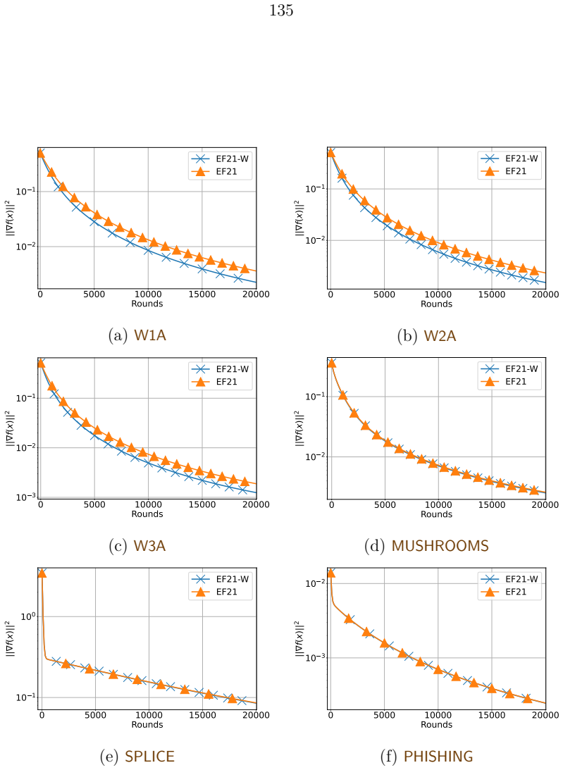
Figure 3.7. Figure 3.7: Non-Convex logistic regression: comparison of EF21 and EF21-W. The used compressor is Top1. The number of clients 𝑛 = 1,000. Regularization term 𝜆 ∑︀𝑑 𝑗=1 𝑥 2 𝑗 𝑥 2 𝑗 + 1 , with 𝜆 = 0.001. Theoretical step size. Full client participation. The objective function is constituted of 𝑓𝑖(𝑥) defined in Equation (3.88). Extra details are in [PITH_FULL_IMAGE:figures/full_fig_p135_3_7.png] view at source ↗
Figure 3.8
Figure 3.8. Figure 3.8: Non-Convex logistic regression: comparison of the performance of standard EF21 and EF21-W. The used compressor is Top1. The number of clients 𝑛 = 200. Regularization term 𝜆 ∑︀𝑑 𝑗=1 𝑥 2 𝑗 𝑥 2 𝑗 + 1 , with 𝜆 = 1,000. Theoretical step size. The objective function is constituted of 𝑓𝑖(𝑥) defined in Equation (3.88). Extra details are in [PITH_FULL_IMAGE:figures/full_fig_p136_3_8.png] view at source ↗
Figure 3.9
Figure 3.9. Figure 3.9: Non-Convex logistic regression: comparison of the performance of standard EF21 and EF21-W. The used compressor for EF21 and EF21-W is Natural compressor Horváth et al. (2019). The number of clients 𝑛 = 200. The objective function is constituted of 𝑓𝑖(𝑥) defined in Equation (3.88). Regularization term 𝜆 ∑︀𝑑 𝑗=1 𝑥 2 𝑗 𝑥 2 𝑗 + 1 , with 𝜆 = 1,000. Multipliers of theoretical step size. Full participa￾tion. Co… view at source ↗
Figure 3.10
Figure 3.10. Figure 3.10: Convex smooth optimization. EF21-PP and EF21-W-PP with Top1 client compressor, 𝑛 = 2 000, 𝑑 = 10. The objective function is constituted of 𝑓𝑖(𝑥) defined in Equation (3.89). Regularization term 𝜆 ‖𝑥‖ 2 2 , 𝜆 = 0.01. Theoretical step size. The objective function is constitute of 𝑓𝑖(𝑥) defined in Equation (3.89). Each client participates in each round with probability 𝑝𝑖 = 0.5. Extra details are in [PITH_… view at source ↗
Figure 3.11
Figure 3.11. Figure 3.11: Non-Convex logistic regression: comparison of EF21-PP and EF21-W-PP. The used compressor is Top1. The number of clients 𝑛 = 1,000. Regularization term 𝜆 ∑︀𝑑 𝑗=1 𝑥 2 𝑗 𝑥 2 𝑗 + 1 , 𝜆 = 0.001. Theoretical step size. Each client participates in each round with probability 𝑝𝑖 = 0.5. The objective function is constitute of 𝑓𝑖(𝑥) defined in Equation (3.90). Extra details are in [PITH_FULL_IMAGE:figures/full_f… view at source ↗
Figure 3.12
Figure 3.12. Figure 3.12: Non-Convex logistic regression: comparison of EF21-PP and EF21-W-PP. The used compressor is Top1. The number of clients 𝑛 = 200. Regularization term 𝜆 ∑︀𝑑 𝑗=1 𝑥 2 𝑗 𝑥 2 𝑗 + 1 , with 𝜆 = 1,000. Theoretical step size. Each client participates in each round with probability 𝑝𝑖 = 0.5. The objective function is constitute of 𝑓𝑖(𝑥) defined in Equation (3.90). Extra details are in [PITH_FULL_IMAGE:figures/ful… view at source ↗
Figure 3.13
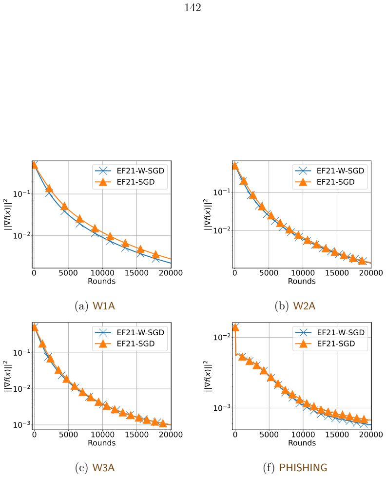
Figure 3.13. Figure 3.13: Non-Convex logistic regression: comparison of EF21-SGD and EF21- W-SGD. The used compressor is Top1. The SGD gradient estimator is SGD-US, 𝜏 = 1. The number of clients 𝑛 = 1,000. The objective function is constitute of 𝑓𝑖(𝑥) defined in Equation (3.91). Regularization term 𝜆 ∑︀𝑑 𝑗=1 𝑥 2 𝑗 𝑥 2 𝑗 + 1 , 𝜆 = 0.001. Theoretical step size. See also [PITH_FULL_IMAGE:figures/full_fig_p142_3_13.png] view at source ↗
Figure 3.14
Figure 3.14. Figure 3.14: Non-Convex logistic regression: comparison of EF21-SGD and EF21- W-SGD. The used compressor is Top1. The SGD gradient estimator is SGD-US, 𝜏 = 1. The number of clients 𝑛 = 200. The objective function is constitute of 𝑓𝑖(𝑥) defined in Equation (3.91). Regularization term 𝜆 ∑︀𝑑 𝑗=1 𝑥 2 𝑗 𝑥 2 𝑗 + 1 , with 𝜆 = 1,000. Theoretical step size. Full participation. Extra details are in [PITH_FULL_IMAGE:figures/f… view at source ↗
Figure 4.1
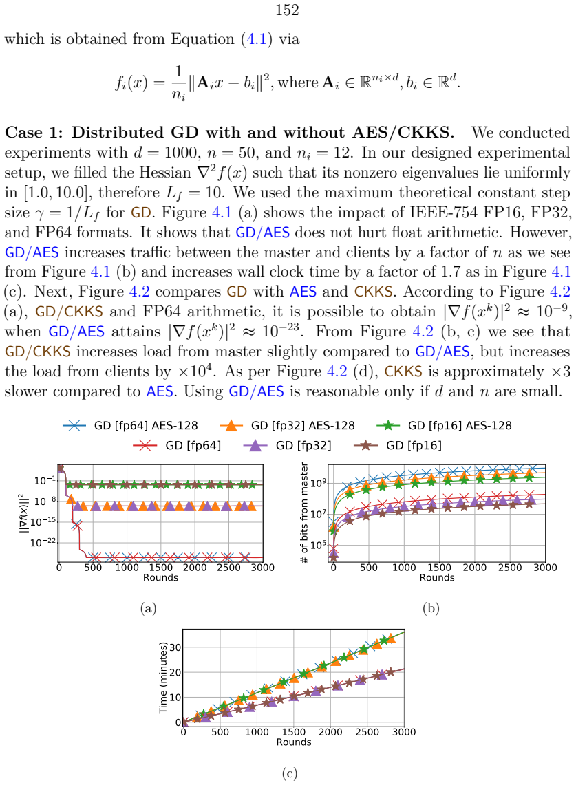
Figure 4.1. Figure 4.1: Synthesized linear regression in interpolation mode, 𝑛𝑖 = 12, 𝑛 = 50, 𝑑 = 1000. No compression. Theoretical step sizes. Case 2: DCGD with AES/CKKS. In this experiment, we employ DCGD with RandK sparsification compressor to analyze the possibility of gradient sparsification while preserving the client’s privacy from the master. To compress ∇𝑓𝑖(𝑥) each client creates a set 𝑆𝑖 ⊂ {1,2, . . . ,𝑑} of size 𝐾 ch… view at source ↗
Figure 4.2
Figure 4.2. Figure 4.2: Synthesized linear regression in interpolation mode, 𝑛𝑖 = 12, 𝑛 = 50, 𝑑 = 1000. No compression. Theoretical step sizes. basis of R 𝑑 . Results are presented in [PITH_FULL_IMAGE:figures/full_fig_p153_4_2.png] view at source ↗
Figure 4.3
Figure 4.3. Figure 4.3: Synthesized linear regression in interpolation, 𝑛𝑖 = 12, 𝑛 = 50, 𝑑 = 1000. Compressors: RandK[𝐾 = 0.2𝑑]. Theoretical step sizes. computed 𝑏𝑖 def = A𝑖𝑥fixed. We tested various step sizes demonstrated in [PITH_FULL_IMAGE:figures/full_fig_p154_4_3.png] view at source ↗
Figure 4.4
Figure 4.4. Figure 4.4: Synthesized linear regression in interpolation, 𝑛𝑖 = 12, 𝑛 = 50, 𝑑 = 1000. Compressors: RandK [𝐾 = 0.2𝑑]. Theoretical step sizes. 0 5000 10000 15000 20000 25000 30000 Rounds 0 5000 10000 15000 20000 25000 30000 Rounds = 1e 05 = 3e 05 = 5e 05 = 7e 05 = 0.0003 = 0.001 = 0.003 = 0.005 = 0.007 = 0.01 = 0.05 0 5000 10000 15000 20000 25000 30000 Rounds 0 5000 10000 15000 20000 25000 30000 Rounds = 1e 05 = 3e 0… view at source ↗
Figure 4.5
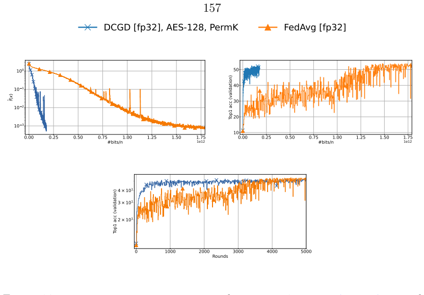
Figure 4.5. Figure 4.5: Tuning step size 𝛾 without decay for DCGD/PermK. Synthesized linear regression in interpolation, 5 launches, FP64. 4.4.2 Image classification application We evaluated the applicability of using DCGD/PermK/AES on Deep Neural Networks training. We used the ResNet-18 architecture (He et al., 2016) and trained it on CIFAR-10 dataset (Krizhevsky and Hinton, 2009), which consists of 60 000 [PITH_FULL_IMAGE:fi… view at source ↗
Figure 4.6
Figure 4.6. Figure 4.6: Linear regression in an interpolation. DCGD uses tuned step size. GD, GD/CKKS, GD/AES use theoretical. images across 10 classes with a resolution of 32 × 32 pixels. We used ResNet-18 implementation from TorchVision library, part of PyTorch (Paszke et al., 2019). The model size 𝑑 = 11,181,642. For Optimization Problem (4.1), we used a standard cross-entropy loss for ℒ𝑖𝑗 terms in Equation (4.2). Next, we d… view at source ↗
Figure 4.7
Figure 4.7. Figure 4.7: ResNet-18 in CIFAR-10, 𝑛 = 10, 𝑑 = 11 181 642. DCGD/PermK/AES and FedAVG. 4.5 Deployment Flexibility The physical network topologies describe the arrangement of the computation and routing devices. In a mesh topology, every pair of nodes is connected with a dedicated link. It has high bandwidth and fault tolerance but requires a lot of cables. In this setting, DCGD/PermK is the natural choice. The Algori… view at source ↗
Figure 4.8
Figure 4.8. Figure 4.8: A high-level view of operations inside the [PITH_FULL_IMAGE:figures/full_fig_p186_4_8.png] view at source ↗
Figure 4.9
Figure 4.9. Figure 4.9: shows that the CKKS overhead from encryption is ×103 more both in master to the client, and the client to master communication direction compared to DCGD/PermK/AES. With 𝑑 = 106 the memory footprint for CKSS configured to guarantee the same guarantees as AES-128 in the master to store 𝑛 = 50 encrypted gradients is 46 GBytes, rendering storage of such information in the master challenging. The best conver… view at source ↗
Figure 4.10
Figure 4.10. Figure 4.10: Event-based modeling for training linear regression across 𝑛 = 4 clients, 𝑑 = 10 · 106 , 𝑛1 = 55000, 𝑛2 = 𝑛3 = 𝑛4 = 11000 during 4 rounds. The uplink and downlink bandwidth is 41.54 MBps, latency 28ms, and computational throughput of modeled CPUs is 238.41 GFLOPS. Legend: - Computation and local memory access using all available CPU cores, - Client to master communication (Clients share the same bottlen… view at source ↗
Figure 5.1
Figure 5.1. Figure 5.1: Comparison of samplings and methods on quadratic optimization [PITH_FULL_IMAGE:figures/full_fig_p214_5_1.png] view at source ↗
Figure 5.3
Figure 5.3. Figure 5.3: Comparison of samplings on non-convex machine learning tasks with [PITH_FULL_IMAGE:figures/full_fig_p214_5_3.png] view at source ↗
Figure 5.2
Figure 5.2. Figure 5.2: Comparison of samplings and methods on quadratic optimization [PITH_FULL_IMAGE:figures/full_fig_p215_5_2.png] view at source ↗
Figure 5.4
Figure 5.4. Figure 5.4: Comparison of samplings and methods with various batch sizes. The [PITH_FULL_IMAGE:figures/full_fig_p217_5_4.png] view at source ↗
Figure 5.5
Figure 5.5. Figure 5.5: The distribution of Lipschitz constants 𝐿𝑖 [PITH_FULL_IMAGE:figures/full_fig_p217_5_5.png] view at source ↗
Figure 5.6
Figure 5.6. Figure 5.6: Comparison of methods on AUSTRALIAN dataset from LIBSVM [PITH_FULL_IMAGE:figures/full_fig_p219_5_6.png] view at source ↗
Figure 6.1
Figure 6.1. Figure 6.1: Training 𝑛 local devices, {𝑊𝑖} on the loss, 𝑓𝑖 of their local model, 𝑥𝑖 with a central server/master node, where ℎ𝑖 penalizes for dissimilarity between the local model, 𝑥𝑖 and the average of all local models, 𝑥. ¯ Device 1 Device 2 Toss a coin 𝑥! " 𝑥! # 𝑥̅ 𝑥" $ 𝑥# $ Device 1 Device 2 𝛼𝜆 𝑛𝑝 𝛼𝜆 𝑛𝑝 1 − 𝛼𝜆 𝑛𝑝 1 − 𝛼𝜆 𝑛𝑝 Device 1 Device 2 Time steps, 𝑇 > 0 𝑥! " 𝑥! # 𝑥! $ Device 1 Device 2 (a) FedAVG Device 1 D… view at source ↗
Figure 6.2
Figure 6.2. Figure 6.2: The FedAVG (McMahan et al., 2017) and L2GD (Hanzely and Richtárik, 2020) algorithm on 2 devices. Unlike FedAVG, L2GD does not communicate after a fixed 𝑇 local steps, it communicates based on a probabilistic protocol [PITH_FULL_IMAGE:figures/full_fig_p237_6_2.png] view at source ↗
Figure 6.3
Figure 6.3. Figure 6.3: Uncompressed L2GD on 𝑛 = 5 workers. We show the loss, 𝑓 as a function of 𝑝 and 𝜆 obtained after 𝐾 = 100 iterations of Algorithm 15 with 𝒞 an identity compressor. (a) A1A dataset, 𝑑 = 124,𝜆 = 10, (b) A2A dataset, 𝑑 = 124,𝜆 = 10, (c) A1A dataset, 𝑑 = 124,𝑝 = 0.65 (d) A2A dataset, 𝑑 = 124,𝑝 = 0.65. 6.4.2 Auxiliary results Before we state our main convergence theorem, we state several intermediate results ne… view at source ↗
Figure 6.4
Figure 6.4. Figure 6.4: Training ResNet-18 on CIFAR-10 with 𝑛 = 10 workers. Plots (a)–(d) show behavior on the train set, while (e)–(h) show behavior on the test set [PITH_FULL_IMAGE:figures/full_fig_p255_6_4.png] view at source ↗
Figure 6.5
Figure 6.5. Figure 6.5: Training DenseNet-121 on CIFAR-10 with 𝑛 = 10 workers. Plots (a)–(d) show behavior on the train set, while (e)–(h) show behavior on the test set [PITH_FULL_IMAGE:figures/full_fig_p256_6_5.png] view at source ↗
Figure 6.6
Figure 6.6. Figure 6.6: Training MobileNet on CIFAR-10 with 𝑛 = 10 workers. Plots (a)–(d) show behavior on the train set, while (e)–(h) show behavior on the test set [PITH_FULL_IMAGE:figures/full_fig_p257_6_6.png] view at source ↗
Figure 6.7
Figure 6.7. Figure 6.7: The FedAVG as a particular case of L2GD: Test and train accuracy for ResNet-56 on CIFAR-10. 0 1 2 3 4 5 #bits/n 1e9 2 2.1 2.1 2.2 2.2 2.2 2.3 2.4 f ( x ) FEDAVG(° = 0:01; local epochs = 3) train FEDAVG(° = 0:01; local epochs = 3) test L2GD(´ = 0:5; ¸ = 100:0; p = 0:5; Bernoullip = 1:0) train L2GD(´ = 0:5; ¸ = 100:0; p = 0:5; Bernoullip = 1:0) test [PITH_FULL_IMAGE:figures/full_fig_p258_6_7.png] view at source ↗
Figure 6.8
Figure 6.8. Figure 6.8: The FedAVG as a particular case of L2GD: Test and train loss for ResNet-56 on CIFAR-10 [PITH_FULL_IMAGE:figures/full_fig_p258_6_8.png] view at source ↗
Figure 6.9
Figure 6.9. Figure 6.9: Training ResNet-18 on CIFAR-10, with 𝑛 = 10 workers. Loss and Top-1 accuracy on the train (a)–(b) and test data (c)–(d). 0 20000 Rounds 1 2 f ( x ) FEDOPT(´ = 0:1) L2GDA(´ = 2:0; ¸ = 0:25; p = 0:3; TopK[k = 0:05D]) L2GDB(´ = 2:0; ¸ = 0:25; p = 0:3; Bernoulli[p = 0:85]) L2GDC(´ = 2:0; ¸ = 0:25; p = 0:3; Natural) L2GDD(´ = 2:0; ¸ = 0:25; p = 0:3; QSGD[l = 5]) 0 20000 Rounds 1 2 f ( x ) FEDOPT(´ = 0:1) L2GD… view at source ↗
Figure 6.10
Figure 6.10. Figure 6.10: Training DenseNet-121 on CIFAR-10, with 𝑛 = 10 workers. Loss and Top-1 accuracy on the train (a)–(b), and test data (c)–(d) [PITH_FULL_IMAGE:figures/full_fig_p270_6_10.png] view at source ↗
Figure 6.11
Figure 6.11. Figure 6.11: Training MobileNet on CIFAR-10, with 𝑛 = 10 workers. Loss and Top-1 accuracy on the train (a)–(b), and test data (c)–(d) [PITH_FULL_IMAGE:figures/full_fig_p271_6_11.png] view at source ↗
Figure 7.1
Figure 7.1. Figure 7.1: Discrepancy between worst-case 𝛼 and 𝛼(𝑥) when 𝑥 ∼u.a.r. 𝑆 𝑑−1 . Number of trials 20 000. 𝑘 components. Similarly, choosing 𝜏𝑑 small enough such that 𝑦𝑑 + 𝜏𝑑 ≤ 𝑦𝑘 ensures that 𝑦𝑑 remains in the smallest 𝑑 − 𝑘 components. However, this implies that 𝛼(𝑧) < 𝛼(𝑦), which contradicts the assumption that 𝑦 was the minimizer. Therefore, the assumption that 𝑦 is the minimizer must be false. Consequently, the opti… view at source ↗
Figure 7.2
Figure 7.2. Figure 7.2: FedNL-LS simulation in a single-node, 1000 rounds, theoretical step size, FP64. Line search parameters 𝑐 = 0.49,𝛾 = 0.5. Dataset W8A (49749 samples) augmented with intercept split to 𝑛𝑖 = 350 samples/client. The results of an experiment using FedNL-LS which represent a modification of FedNL are presented in Figures 7.2, 7.3, 7.4. For a pseudocode of FedNL-LS see Appendix A7.1. The communicated bits inclu… view at source ↗
Figure 7.3
Figure 7.3. Figure 7.3: FedNL-LS simulation in a single-node, 1000 rounds, theoretical step size, FP64. Line search parameters 𝑐 = 0.49,𝛾 = 0.5. Dataset A9A (32561 samples) augmented with intercept, split to 𝑛𝑖 = 229 samples/client. 0.0 0.2 0.4 0.6 0.8 1.0 #bits/n 1e7 1e-16 1e-13 1e-10 1e-07 0.0001 k r f ( x t ) k PHISHING d = 69; n = 142; ni = 77; ¸ = 0:001 FedNL-LS (b) Identical FedNL-LS (b) Natural FedNL-LS (b) RandK[k=8d] F… view at source ↗
Figure 7.4
Figure 7.4. Figure 7.4: FedNL-LS simulation in a single-node, 2000 rounds, theoretical step size, FP64. Line search parameters 𝑐 = 0.49,𝛾 = 0.5. Dataset PHISHING ( 11055 samples) augmented with intercept split to 𝑛𝑖 = 77 samples/client [PITH_FULL_IMAGE:figures/full_fig_p307_7_4.png] view at source ↗
Figure 7.5
Figure 7.5. Figure 7.5: FedNL in multi-node setting, theoretical step size, 𝑛 = 50, FP64 arithmetic, 1 CPU core per node and master, TCP/IPv4, dataset W8A reshuffled u.a.r. and augmented with intercept. We have carried out experiments with FedNL, FedNL-LS, and with FedNL-PP FedNL-PP. The results for W8A are presented in Figures 7.5, 7.6, 7.7, for A9A in Figures 7.8, 7.9, 7.10, for PHISHING in Figures 7.11, 7.12, 7.13. In this e… view at source ↗
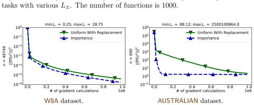
Figure 7.6
Figure 7.6. Figure 7.6: FedNL-LS in multi-node setting, 𝑛 = 50, FP64 arithmetic, 1 CPU core per node and master, TCP/IPv4, dataset W8A reshuffled u.a.r. and augmented with intercept. The line search parameters 𝑐 = 0.49,𝛾 = 0.5. most economical method for sending information from client to master. While it did not enhance TopK when measuring progress in terms of communicated bits, it demonstrated improvement when measuring actua… view at source ↗
Figure 7.7
Figure 7.7. Figure 7.7: FedNL-PP in multi-node setting, 𝑛 = 50, |𝑆 𝑘 | = 12 clients per round, FP64 arithmetic, 1 CPU core per node and master, TCP/IPv4. W8A dataset reshuffled u.a.r. and augmented with intercept. 0 5 10 15 20 25 Elapsed Time (seconds) 1e-15 1e-11 1e-07 0.001 k r f ( x t ) k d = 124; n = 50; ni = 651; ¸ = 0:001 FedNL (b) Natural FedNL (b) RandK[k=8d] FedNL (b) RandSeqK[k=8d] FedNL (b) TopK[k=8d] FedNL (b) TopLE… view at source ↗
Figure 7.8
Figure 7.8. Figure 7.8: FedNL in multi-node setting, theoretical step size, 𝑛 = 50, FP64 arithmetic, 1 CPU core per node and master, TCP/IPv4, dataset A9A reshuffled u.a.r. and augmented with intercept [PITH_FULL_IMAGE:figures/full_fig_p310_7_8.png] view at source ↗
Figure 7.9
Figure 7.9. Figure 7.9: FedNL-LS in multi-node setting, 𝑛 = 50, FP64 arithmetic, 1 CPU core per node and master, TCP/IPv4, dataset A9A reshuffled u.a.r. and augmented with intercept. The line search parameters 𝑐 = 0.49,𝛾 = 0.5. 0 1 2 3 4 5 Elapsed Time (seconds) 1e-13 1e-10 1e-07 0.0001 0.1 k r f ( x t ) k d = 124; n = 50; ni = 651; ¸ = 0:001 FedNL-PP (b) Natural FedNL-PP (b) RandK[k=8d] FedNL-PP (b) RandSeqK[k=8d] FedNL-PP (b)… view at source ↗
Figure 7.10
Figure 7.10. Figure 7.10: FedNL-PP at A9A in multi-node setting, 𝑛 = 50, |𝑆 𝑘 | = 12 clients per round, FP64 arithmetic, 1 CPU core per node and master, TCP/IPv4. A9A dataset reshuffled u.a.r. and augmented with intercept [PITH_FULL_IMAGE:figures/full_fig_p311_7_10.png] view at source ↗
Figure 7.11
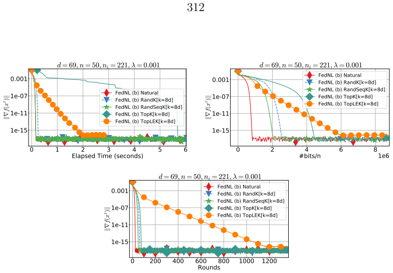
Figure 7.11. Figure 7.11: FedNL in multi-node setting, theoretical step size, 𝑛 = 50, FP64 arith￾metic, 1 CPU core per node and master, TCP/IPv4, dataset PHISHING reshuffled u.a.r. and augmented with intercept. 0 1 2 3 4 5 Elapsed Time (seconds) 1e-15 1e-11 1e-07 0.001 k r f ( x t ) k d = 69; n = 50; ni = 221; ¸ = 0:001 FedNL-LS (b) Natural FedNL-LS (b) RandK[k=8d] FedNL-LS (b) RandSeqK[k=8d] FedNL-LS (b) TopK[k=8d] FedNL-LS (b)… view at source ↗
Figure 7.12
Figure 7.12. Figure 7.12: FedNL-LS in multi-node setting, 𝑛 = 50, FP64 arithmetic, 1 CPU core per node and master, TCP/IPv4, dataset PHISHING reshuffled u.a.r. and augmented with intercept. The line search parameters 𝑐 = 0.49,𝛾 = 0.5 [PITH_FULL_IMAGE:figures/full_fig_p312_7_12.png] view at source ↗
Figure 7.13
Figure 7.13. Figure 7.13: FedNL-PP in multi-node setting, 𝑛 = 50, |𝑆 𝑘 | = 12 clients per round, FP64 arithmetic, 1 CPU core per node and master, TCP/IPv4. PHISHING dataset reshuffled u.a.r. and augmented with intercept [PITH_FULL_IMAGE:figures/full_fig_p313_7_13.png] view at source ↗
Figure 8.1
Figure 8.1. Figure 8.1: Tiny compute graph with 10 nodes to evaluate 𝑔 = 𝑓/2,𝑓 = 𝑒 2 ,𝑒 = 𝑐 − 𝑑, 𝑑 = 𝑎𝑏 + 𝑏 3 , 𝑐 = 𝑎 + 𝑏,𝑎 = −41,𝑏 = 2. Nodes contain: description, operator, ∂𝑔 ∂[node] , value, raw index. The numerical results across frameworks match exactly. 8.2.2 Small compute graph In this experiment, we evaluate the performance of various frameworks on a small computation graph in [PITH_FULL_IMAGE:figures/full_fig_p347_8_1.png] view at source ↗
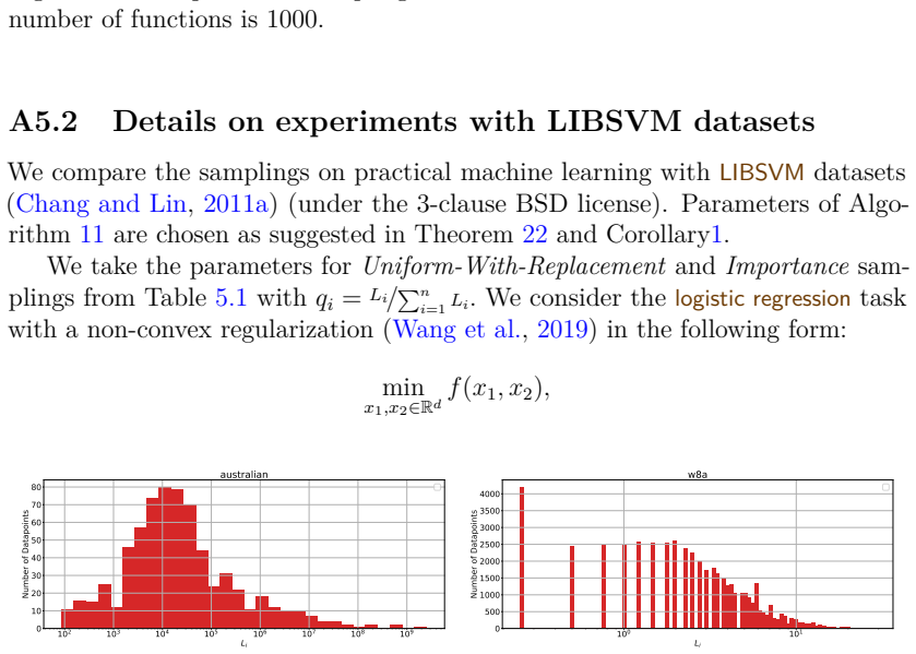
Figure 8.2
Figure 8.2. Figure 8.2: Small compute graph with total 𝑉 = 32 nodes and 𝐸 = 44 edges to evaluate function from Karpathy (2020) [PITH_FULL_IMAGE:figures/full_fig_p348_8_2.png] view at source ↗
Figure 8.3
Figure 8.3. Figure 8.3: Visualization of Table [PITH_FULL_IMAGE:figures/full_fig_p349_8_3.png] view at source ↗
Figure 8.4
Figure 8.4. Figure 8.4: Listings for the small compute graph shown in Figure [PITH_FULL_IMAGE:figures/full_fig_p380_8_4.png] view at source ↗
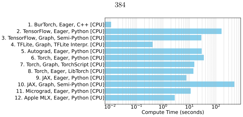
Figure 8.5
Figure 8.5. Figure 8.5: Visualization of Table [PITH_FULL_IMAGE:figures/full_fig_p384_8_5.png] view at source ↗
Figure 8.6
Figure 8.6. Figure 8.6: Visualization of Table [PITH_FULL_IMAGE:figures/full_fig_p387_8_6.png] view at source ↗
Figure 8.7
Figure 8.7. Figure 8.7: Visualization of Table [PITH_FULL_IMAGE:figures/full_fig_p391_8_7.png] view at source ↗

discussion (0)

Sign in with ORCID, Apple, or X to comment. Anyone can read and Pith papers without signing in.

Reference graph

Works this paper leans on

16 extracted references · 6 canonical work pages

  1. [5]

    arXiv:2110.03294 https: //arxiv.org/abs/2110.03294 Ilyas Fatkhullin, Alexander Tyurin, and Peter Richtárik

    EF21 with Bells & Whistles: Practical Algorithmic Extensions of Modern Error Feedback.CoRRabs/2110.03294 (2021). arXiv:2110.03294 https: //arxiv.org/abs/2110.03294 Ilyas Fatkhullin, Alexander Tyurin, and Peter Richtárik. 2023. Momentum Prov- ably Improves Error Feedback!. InAdvances in Neural Information Processing Systems 36: Annual Conference on Neural ...

  2. [7]

    MLX: Efficient and flexible machine learning on Apple silicon.https: //github.com/ml-explore Filip Hanzely and Peter Richtárik. 2020. Federated Learning of a Mixture of Global and Local Models.CoRRabs/2002.05516 (2020). arXiv:2002.05516 https://arxiv.org/abs/2002.05516 Andrew Hard, Kanishka Rao, Rajiv Mathews, Françoise Beaufays, Sean Au- genstein, Hubert...

  3. [8]

    In2017 IEEE Conference on Computer Vision and Pattern Recognition, CVPR 2017, Honolulu, HI, USA, July 21-26, 2017

    Densely Connected Convolutional Networks. In2017 IEEE Conference on Computer Vision and Pattern Recognition, CVPR 2017, Honolulu, HI, USA, July 21-26, 2017. IEEE Computer Society, 2261–2269.https://doi.org/10. 1109/CVPR.2017.243 Junxian Huang, Feng Qian, Yihua Guo, Yuanyuan Zhou, Qiang Xu, Zhuoqing Mor- ley Mao, Subhabrata Sen, and Oliver Spatscheck. 2013...

  4. [11]

    Randomized Automatic Differentiation. (2021). https://openreview. net/forum?id=xpx9zj7CUlY Ceylan Onay and Elif Öztürk. 2018. A review of credit scoring research in the age of Big Data.Journal of Financial Regulation and Compliance26, 3 (2018), 382–405. Owkin. 2020. Story of the 1st Federated Learning Model at Owkin. https: //owkin.com/federated-learning/...

  5. [13]

    70), Doina Precup and Yee Whye Teh (Eds.)

    DistributedMeanEstimationwithLimitedCommunication.InProceedings 434 of the 34th International Conference on Machine Learning, ICML 2017, Sydney, NSW, Australia, 6-11 August 2017 (Proceedings of Machine Learning Research, Vol. 70), Doina Precup and Yee Whye Teh (Eds.). PMLR, 3329–3337.http: //proceedings.mlr.press/v70/suresh17a.html Rafal Szlendak, Alexand...

  6. [14]

    Sharper Rates and Flexible Framework for Nonconvex SGD with Client and Data Sampling.Trans. Mach. Learn. Res.2023 (2023). https: //openreview.net/forum?id=zKgJ6TWAFE C. H. van Berkel. 2009. Multi-core for mobile phones. InDesign, Automation and Test in Europe, DATE 2009, Nice, France, April 20-24, 2009, Luca Benini, Giovanni De Micheli, Bashir M. Al-Hashi...

  7. [15]

    InProceedings of the 2020 USENIX Annual Technical Con- ference, USENIX ATC 2020, July 15-17, 2020, Ada Gavrilovska and Erez Zadok (Eds.)

    BatchCrypt: Efficient Homomorphic Encryption for Cross-Silo Feder- ated Learning. InProceedings of the 2020 USENIX Annual Technical Con- ference, USENIX ATC 2020, July 15-17, 2020, Ada Gavrilovska and Erez Zadok (Eds.). USENIX Association, 493–506. https://www.usenix.org/ conference/atc20/presentation/zhang-chengliang Hantian Zhang, Jerry Li, Kaan Kara, D...

  8. [16]

    In 9th International Conference on Learning Representations, ICLR 2021, Virtual Event, Austria, May 3-7, 2021

    Personalized Federated Learning with First Order Model Optimization. In 9th International Conference on Learning Representations, ICLR 2021, Virtual Event, Austria, May 3-7, 2021. OpenReview.net.https://openreview.net/ forum?id=ehJqJQk9cw Sixin Zhang, Anna Choromanska, and Yann LeCun. 2015. Deep learning with Elastic Averaging SGD. InAdvances in Neural In...

  9. [1999]

    In40th Annual Symposium on Foundations of Computer Science, FOCS ’99, 17-18 October, 1999, New York, NY, USA

    Cache-Oblivious Algorithms. In40th Annual Symposium on Foundations of Computer Science, FOCS ’99, 17-18 October, 1999, New York, NY, USA. IEEE Computer Society, 285–298. https://doi.org/10.1109/SFFCS.1999. 814600 Rishikesh R. Gajjala, Shashwat Banchhor, Ahmed M. Abdelmoniem, Aritra Dutta, Marco Canini, and Panos Kalnis. 2020. Huffman Coding Based Encoding...

  10. [2017]

    (2017), 1709–1720

    QSGD: Communication-Efficient SGD via Gradient Quantization and Encoding. (2017), 1709–1720. https://proceedings.neurips.cc/paper/ 2017/hash/6c340f25839e6acdc73414517203f5f0-Abstract.html Dan Alistarh, Torsten Hoefler, Mikael Johansson, Nikola Konstantinov, Sarit Khirirat, and Cédric Renggli. 2018. The Convergence of Sparsified Gradient Methods. InAdvance...

  11. [2019]

    arXiv:1901.09269 http://arxiv.org/abs/1901

    Distributed Learning with Compressed Gradient Differences.CoRR abs/1901.09269 (2019). arXiv:1901.09269 http://arxiv.org/abs/1901. 09269 Konstantin Mishchenko, Grigory Malinovsky, Sebastian U. Stich, and Peter Richtárik. 2022. ProxSkip: Yes! Local Gradient Steps Provably Lead to Communication Acceleration! Finally!. InInternational Conference on Machine Le...

  12. [2020]

    Secure, privacy-preserving and federated machine learning in medical imaging.Nat. Mach. Intell.2, 6 (2020), 305–311. https://doi.org/10.1038/ S42256-020-0186-1 Sai Praneeth Karimireddy, Satyen Kale, Mehryar Mohri, Sashank J. Reddi, Se- bastian U. Stich, and Ananda Theertha Suresh. 2020. SCAFFOLD: Stochastic Controlled Averaging for Federated Learning. InP...

  13. [2021]

    ACM, 1–7.https://doi.org/10.1145/3488659.3493775 Konstantin Burlachenko and Peter Richtárik. 2024. Unlocking FedNL: Self- Contained Compute-Optimized Implementation.CoRRabs/2410.08760 (2024). https://doi.org/10.48550/ARXIV.2410.08760arXiv:2410.08760 Konstantin Burlachenko and Peter Richtárik. 2025. BurTorch: Revisiting Training from First Principles by Co...

  14. [2022]

    RevEAL: Single-Trace Side-Channel Leakage of the SEAL Homomorphic Encryption Library. In2022 Design, Automation & Test in Europe Conference & Exhibition, DATE 2022, Antwerp, Belgium, March 14-23, 2022, Cristiana Bolchini, Ingrid Verbauwhede, and Elena-Ioana Vatajelu (Eds.). IEEE, 1527– 1532.https://doi.org/10.23919/DATE54114.2022.9774724 Boaz Barak, Oded ...

  15. [2023]

    Personalized Federated Learning with Communication Compression. Trans. Mach. Learn. Res.2023 (2023).https://openreview.net/forum?id= dZugyhbNFY James Bergstra, Olivier Breuleux, Frédéric Bastien, Pascal Lamblin, Razvan Pascanu, Guillaume Desjardins, Joseph P. Turian, David Warde-Farley, and Yoshua Bengio. 2010. Theano: A CPU and GPU Math Compiler in Pytho...

  16. [2024]

    Yang, Zachary DeVito, Martin Raison, Alykhan Tejani, Sasank Chilamkurthy, Benoit Steiner, Lu Fang, Junjie Bai, and Soumith Chintala

    FedSHE: privacy preserving and efficient federated learning with adaptive segmented CKKS homomorphic encryption.Cybersecur.7, 1 (2024), 40.https: //doi.org/10.1186/S42400-024-00232-W Adam Paszke, Sam Gross, Francisco Massa, Adam Lerer, James Bradbury, Gregory Chanan, Trevor Killeen, Zeming Lin, Natalia Gimelshein, Luca Antiga, Alban Desmaison, Andreas Köp...