REVIEW 3 major objections 6 minor 23 references
OCTANE frames autoencoder training as an optimal control problem, letting layer widths emerge from tensor rank truncation.
Reviewed by Pith at T0; open to challenge. T0 means a machine referee read the full paper against a public rubric. the ladder, T0–T4 →
Autoencoders as continuous-time optimal control problems solved with rank-adaptive tensor compression, yielding memory savings and automatic layer-width profiles on MNIST denoising and deblurring.
T0 review reviewed 2026-08-04 challenge →
load-bearing objection A promising but under-supported combination of optimal control and tensor ranks; the numerical error analysis does not cover the actual experimental setup. the 3 major comments →
OCTANE -- Optimal Control for Tensor-based Autoencoder Network Emergence: Explicit Case
The pith
A machine-rendered reading of the paper's core claim, the machinery that carries it, and where it could break.
The reading
Core claim
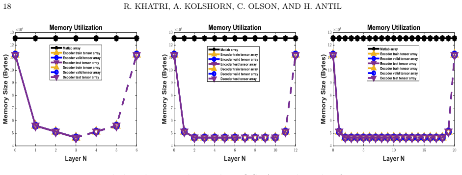
On its own terms, the paper claims that compression in an autoencoder does not have to be imposed by a preset layer-width schedule. In the OCTANE formulation the encoder and decoder are the forward solutions of two coupled ODEs, and each explicit Euler step is rounded to a tensor-train manifold by truncation operators whose tolerances are set by local error bounds. The sequence of selected ranks is then read as the discovered architecture: the rank profile literally gives the layer widths and produces a butterfly-shaped structure. The paper also claims the resulting discrete optimality system is differentiable in the right sense — gradient checks against finite differences pass at the expect
What carries the argument
The load-bearing object is the rank-adaptive explicit Euler integrator applied to tensor-valued ODEs: at each step the right-hand side is first truncated by an operator T_s and the updated state is then truncated by T_r, with tolerances chosen through the error bounds (3a)-(3b) and (6a)-(6b). Working in the tensor-train format — a low-rank decomposition that stores a high-order array through a chain of small core tensors — this single mechanism performs three jobs at once: it discretizes the continuous optimal control ODEs, it keeps the state and adjoint trajectories low-rank, and it generates the rank profile that defines the autoencoder architecture. The reverse-time version of the same sc
Load-bearing premise
The whole scheme depends on the assumption that the rank-truncated explicit Euler steps stay first-order accurate for the coupled state and adjoint optimality system when truncation tolerances are chosen at the aggressive scales used in the experiments; the paper proves one-step local error bounds but not convergence of the full algorithm.
What would settle it
Fix T and run the full OCTANE training loop at decreasing τ (increasing layer count N), and compare the discrete gradient computed by the paper's training procedure to a finite-difference gradient of the same discrete loss. If the mismatch does not fall at roughly first order as τ shrinks, or plateaus because rank truncation dominates, the order-one consistency claim fails.
If this is right
- Layer widths stop being a hyperparameter: the truncation-selected ranks during forward integration define the discovered autoencoder architecture.
- Memory use is tied to tensor ranks rather than full data dimensions; the experiments report average savings of about 7–16% for denoising and 47–57% for deblurring on the tested MNIST tasks.
- Training is feasible with very little data: 20 training images sufficed in the reported denoising and deblurring runs.
- A practical operating window for the step size and time horizon, roughly 0.3 ≤ τ ≤ 1.3 with T ∈ {10, 15}, is recommended for consistent performance at lower cost.
Where Pith is reading between the lines
- The rank-profile view suggests a cheap architecture-search alternative: instead of training many candidate widths, one could train once and read the widths off the rank curve; whether this profile is stable across random initializations is a direct test the paper does not report.
- Because the integration scheme is described as agnostic to the tensor format, the framework should extend to Tucker or HOSVD decompositions; a testable prediction is that equivalent rank profiles and reconstruction quality would emerge in any fixed low-rank format.
- The paper imposes a symmetric encoder-decoder by setting r_d = flip(r_e); relaxing that symmetry could expose tasks where the encoder needs more capacity than the decoder, and whether the butterfly shape is optimal is left open.
- The memory savings are reported for the state variables; an end-to-end accounting that includes adjoint trajectories and optimizer state would clarify the true practical gain.
Editorial analysis
A structured set of objections, weighed in public.
Referee Report
Summary. The manuscript proposes OCTANE, an autoencoder framework in which the encoder and decoder are defined by coupled ODEs and trained as an optimal control problem. A Lagrangian derivation gives first-order necessary conditions (state, adjoint, and design equations), and the state/adjoint systems are discretized with a rank-adaptive explicit Euler scheme on tensor-train manifolds. The algorithm stores encoder ranks during forward propagation, imposes decoder ranks as the reversal of encoder ranks, and trains with a gradient-based optimizer. Experiments on MNIST digit denoising and deblurring show reconstructions, rank profiles, memory comparisons, and a recommended step-size/layer-count interval.
Significance. The core idea is attractive: a continuous optimal-control formulation of autoencoders, combined with low-rank tensor integration, could provide a principled way to obtain compact architectures. The Lagrangian derivation in Sections 3–4 is self-contained and standard, and the gradient test in Section 6.1.3 is a useful verification of the discrete gradients. The authors also give enough algorithmic detail to make the experiments reproducible. If the convergence and architecture-discovery claims can be repaired, OCTANE would be a valuable contribution. However, as written, the advertised mathematical rigor and the claim that the architecture is automatically discovered are not supported: the truncation tolerances used in all experiments invalidate the stated first-order consistency, and the decoder rank profile is imposed by symmetry rather than emergent.
major comments (3)
- [Section 2.1, Eqs. (3a)-(3b); Table 2; Section 6.4] The conditions (3a)-(3b) yield a first-order guarantee only when Ms and Mr are fixed constants independent of tau. In Table 2 the authors set Ms=tau^{-1} and Mr=tau^{-2}, so the right-hand sides of (3a) and (3b) become 1 and 1. Writing e_s=N-T_s(N) and e_r=Y_j+tau T_s(N)-T_r(...), the one-step error of (2) is -tau e_s - e_r + O(tau^2), bounded by Ms tau^2 + Mr tau^2 + O(tau^2)=tau+1+O(tau^2)=O(1). Thus the scheme is not shown to be consistent as tau->0, and the discrete optimality system (13)-(15) is not established as a faithful discretization of (10)-(12). Section 6.4 explicitly confirms that this choice decouples the tolerance from tau. Please take Ms,Mr to be O(1) constants independent of tau, or provide a convergence analysis of the full rank-adaptive scheme under the actual parameter choices, and rerun the experiments under conditions where the claimed order holds.
- [Section 5.1(c)-(e); Algorithm 5, line 7] The decoder rank profile is prescribed by r_d=flip(r_e) at Algorithm 5 line 7 and in Section 5.1(c). Consequently only the encoder ranks are selected by the truncation operators; the decoder widths are imposed by symmetry. This contradicts the statement in Section 5.1(e) that the resulting encoder and decoder ranks define the discovered architecture and that the ranks emerge naturally from the dynamics. Please qualify the architecture-discovery claim, or allow the decoder ranks to be chosen independently and test whether a symmetric profile actually emerges.
- [Section 6.4, Eq. (23)] The recommended interval tau_proposed=(0.3,1.3) is obtained by intersecting thresholds (alpha<1e-3, SSIM>=0.96, etc.) on the same experimental runs whose behavior it is meant to predict. This is a fit to the data, not a validated recommendation. Independent hyperparameter validation, such as a separate sweep or cross-validation, is needed before presenting (23)-(24) as guidance. In addition, the experiments report no baselines and no error bars, so the comparative claims of effectiveness and the memory-saving percentages in Sections 6.2-6.3 are not yet established.
minor comments (6)
- [Section 2.1] The phrase 'order one local truncation error' is imprecise: the underlying Euler step has second-order local truncation error and first-order global error. Please correct the terminology.
- [Figure 7 caption] Typo: 'delurring' should be 'deblurring'.
- [Figure 6] The leftmost subplot appears to lack a title or axis label indicating 'Reconstruction Error'; please add it.
- [Algorithms 1-4] The comments state 'Choose smallest s_j>0 s.t. (3a) holds' and 'If not found, break', but no search procedure or fallback is described. Specify how the ranks are determined when the condition is not met.
- [Section 4.1 and Algorithms 1-4] Notation conflict: u_i:=u(t_i) is introduced in Section 4.1, but u is later used for the intermediate update tensor in Algorithms 1-4. Rename one of them to avoid confusion.
- [Equation (22)] For Ms=tau^{-1}, Mr=tau^{-2}, the TT tolerances epsilon become independent of tau. This is directly related to Major Comment 1 and should at least be acknowledged as a limitation of the error control.
Circularity Check
Decoder rank profile is forced by r_d=flip(r_e), so the 'automated architecture discovery' claim is partly definitional; the core optimal-control derivation is self-contained.
specific steps
-
self definitional
[Section 5.1(c) and (e); Algorithm 5 line 7]
"Define r_d := flip(r_e) to impose symmetry across the encoder-decoder interface. ... The resulting vectors of encoder and decoder ranks in forward integration, selected by the truncation operators, define the discovered autoencoder architecture. ... The resultant ranks are not learned via optimization; they emerge naturally from the dynamics of the problem and the input data."
Algorithm 5 line 7 sets r_d <- flip(r_f e), so the decoder rank profile is, by construction, the reverse of the encoder rank profile. The decoder half of the claimed 'discovered autoencoder architecture' therefore carries no independent dynamical information; it is forced to mirror the encoder. The statement that ranks 'emerge naturally from the dynamics of the problem and the input data' is definitionally false for the decoder, making the architecture-discovery claim partially circular. The encoder ranks are still data-dependent, but the full published rank profile is not an emergent output as claimed.
full rationale
The main mathematical derivation is self-contained: the optimal-control formulation, Lagrangian, and state/adjoint/design equations are derived in Section 3 without relying on a load-bearing self-citation; the rank-adaptive Euler scheme is described in Section 2 and attributed to the independent reference [20]. No uniqueness theorem is smuggled in, and no known result is merely renamed. The only significant circularity is the forced decoder rank mirror in Section 5.1(c)/Algorithm 5, which partly undermines the 'automated architecture discovery' claim by defining half of the reported architecture in terms of the other half. The empirical tau-recommendation in Section 6.4 is explicitly presented as a heuristic derived from the plotted experiments and is checked on digit 4, so it is a post-hoc fit rather than a disguised prediction, though it should not be read as a validated general law. The M_s=tau^-1, M_r=tau^-2 choice raises a consistency/correctness issue for the Euler error bounds, but that is a numerical-analysis gap rather than a circular step. Overall score reflects one definitional reduction in a supporting claim, not circularity in the core derivation.
Axiom & Free-Parameter Ledger
free parameters (6)
- Step size tau =
T/N; explored 0.18-3.75; recommended range (0.3,1.3) fitted to data
- Terminal time T =
10 in main experiments; recommended {10,15}
- Number of layers N =
4 to 30 in scans
- Error constants M_s, M_r =
tau^-1, tau^-2 (Table 2)
- Regularization weights lambda1..lambda4 =
1e-5, 1e-5, 1, 1 (denoising); 0, 0, 0.1, 0.1 (deblurring)
- Optimization iterations m1, m2 =
3, 30
axioms (6)
- domain assumption The rank-adaptive Euler scheme from [20] provides a stable, first-order accurate approximation of (1) under conditions (3),(6).
- standard math Tensor-train rounding satisfies ||a - T(a)|| <= eps ||a|| (from [17, Cor. 2.4]).
- standard math The optimal control problem (7) has a stationary point satisfying the first-order necessary conditions (10)-(12).
- domain assumption Using equal numbers of encoder and decoder layers (N_e = N/2) is sufficient for the considered tasks.
- domain assumption BFGS with Armijo line search converges to a stationary point of the discretized problem.
- ad hoc to paper The loose truncation tolerances implied by M_s=tau^-1, M_r=tau^-2 still yield sufficiently accurate solutions and meaningful ranks.
Cite this review
Pith. "Pith review of OCTANE -- Optimal Control for Tensor-based Autoencoder Network Emergence: Explicit Case." pith.science (2026). https://pith.science/paper/4OW5R227
@misc{pith2026250908169,
  author       = {Pith},
  title        = {Pith review of: OCTANE -- Optimal Control for Tensor-based Autoencoder Network Emergence: Explicit Case},
  year         = {2026},
  howpublished = {\url{https://pith.science/paper/4OW5R227}},
  note         = {Machine review of arXiv:2509.08169}
}
read the original abstract
This paper presents a novel, mathematically rigorous framework for autoencoder-type deep neural networks that combines optimal control theory and low-rank tensor methods to yield memory-efficient training and automated architecture discovery. The learning task is formulated as an optimization problem constrained by differential equations representing the encoder and decoder components of the network and the corresponding optimality conditions are derived via a Lagrangian approach. Efficient memory compression is enabled by approximating differential equation solutions on low-rank tensor manifolds using an adaptive explicit integration scheme. These concepts are combined to form OCTANE (Optimal Control for Tensor-based Autoencoder Network Emergence) -- a unified training framework that yields compact autoencoder architectures, reduces memory usage, and enables effective learning, even with limited training data. The framework's utility is illustrated with application to image denoising and deblurring tasks and recommendations regarding governing hyperparameters are provided.
Figures




Reference graph
Works this paper leans on
-
[1]
H. Antil, T. Brown, R. Khatri, A. Onwunta, D. Verma, and M. Warma. Optimal control, numerics, and applica- tions of fractional pdes. In E. Tr´ elat and E. Zuazua, editors,Numerical Control: Part A, volume 23 ofHandbook of Numerical Analysis, pages 87–114. Elsevier, Amsterdam, the Netherlands, 2022
work page 2022
- [2]
-
[3]
Novel Deep neural networks for solving Bayesian statistical inverse
H. Antil, H. C. Elman, A. Onwunta, and D. Verma. Novel deep neural networks for solving bayesian statistical inverse.arXiv preprint arXiv:2102.03974, 2021
work page internal anchor Pith review Pith/arXiv arXiv 2021
- [4]
-
[5]
Tensor Decompositions in Deep Learning
D. Bacciu and D. P. Mandic. Tensor decompositions in deep learning.arXiv preprint arXiv:2002.11835, 2020
work page internal anchor Pith review Pith/arXiv arXiv 2002
-
[6]
D. Bank, N. Koenigstein, and R. Giryes. Autoencoders.arXiv preprint arXiv:2003.05991, 2021
Pith/arXiv arXiv 2003
-
[7]
Neural Architecture Search via Bregman Iterations
L. Bungert, T. Roith, D. Tenbrinck, and M. Burger. Neural architecture search via bregman iterations.arXiv preprint arXiv:2106.02479, 2021
work page internal anchor Pith review Pith/arXiv arXiv 2021
-
[8]
R. T. Q. Chen, Y. Rubanova, J. Bettencourt, and D. Duvenaud. Neural ordinary differential equations.Advances in Neural Information Processing Systems, 2018
work page 2018
-
[9]
X. Glorot and Y. Bengio. Understanding the difficulty of training deep feedforward neural networks. InProceed- ings of the Thirteenth International Conference on Artificial Intelligence and Statistics, volume 9 ofProceedings of Machine Learning Research, pages 249–256, Chia Laguna Resort, Sardinia, Italy, 13–15 May 2010. PMLR
work page 2010
-
[10]
I. Goodfellow, Y. Bengio, and A. Courville.Deep Learning. MIT Press, Massachusetts, USA, 2016.http://www. deeplearningbook.org
work page 2016
-
[11]
S. G¨ unther, L. Ruthotto, J. Schroder, E. Cyr, and N. Gauger. Layer-parallel training of deep residual neural networks.SIAM Journal on Mathematics of Data Science, 2:1–23, 01 2020
work page 2020
-
[12]
C. T. Kelley.Iterative methods for optimization. Frontiers in applied mathematics. SIAM, Philadelphia, USA, 1999. 22 R. KHATRI, A. KOLSHORN, C. OLSON, AND H. ANTIL
work page 1999
-
[13]
Lecun, L
Y. Lecun, L. Bottou, Y. Bengio, and P. Haffner. Gradient-based learning applied to document recognition. Proceedings of the IEEE, 86(11):2278–2324, 1998
1998
-
[14]
N. Merrill and A. Eskandarian. Modified autoencoder training and scoring for robust unsupervised anomaly detection in deep learning.IEEE Access, 8:101824–101833, 2020
work page 2020
-
[15]
N. Merrill and C. C. Olson. A new autoencoder training paradigm for unsupervised hyperspectral anomaly detection. InIGARSS 2020 - 2020 IEEE International Geoscience and Remote Sensing Symposium, pages 3967– 3970, 2020
work page 2020
-
[16]
A. Novikov, D. Podoprikhin, A. Osokin, and D. P Vetrov. Tensorizing neural networks. In C. Cortes, N. Lawrence, D. Lee, M. Sugiyama, and R. Garnett, editors,Advances in Neural Information Processing Systems, volume 28, Montr´ eal, Canada, 2015. Curran Associates, Inc
work page 2015
-
[17]
I. V. Oseledets. Tensor-train decomposition.SIAM Journal on Scientific Computing, 33(5):2295–2317, 2011
2011
-
[18]
I. V. Oseledets, S. Dolgov, V. Kazeev, O. Lebedeva, and T. Mach. Tt-toolbox.https://github.com/oseledets/TT- Toolbox, 2014
work page 2014
-
[19]
P. Peng, S. Jalali, and X. Yuan. Solving inverse problems via auto-encoders.IEEE Journal on Selected Areas in Information Theory, 1(1):312–323, 2020
work page 2020
-
[20]
A. Rodgers, A. Dektor, and D. Venturi. Adaptive integration of nonlinear evolution equations on tensor manifolds. Journal of Scientific Computing, 92(2), jun 2022
work page 2022
-
[21]
R. Salakhutdinov and G. Hinton. Semantic hashing.International Journal of Approximate Reasoning, 50(7):969– 978, July 2009
work page 2009
- [22]
-
[23]
A. Zhavoronkov, Y. A. Ivanenkov, A. Aliper, M. S. Veselov, V. A. Aladinskiy, A. V. Aladinskaya, V. A. Terentiev, D. A. Polykovskiy, M. D. Kuznetsov, A. Asadulaev, Y. Volkov, A. Zholus, R. R. Shayakhmetov, A. Zhebrak, L. I. Minaeva, B. A. Zagribelnyy, L. H. Lee, R. Soll, D. Madge, L. Xing, T. Guo, and A. Aspuru-Guzik. Deep learning enables rapid identifica...
work page 2019
This paper was first reviewed by deepseek-v4-flash on August 4, 2026.
discussion (0)
Sign in with ORCID, Apple, or X to comment. Anyone can read and Pith papers without signing in.