Beyond Spherical geometry: Unraveling complex features of objects orbiting around stars from its transit light curve using deep learning
Pith reviewed 2026-05-18 16:11 UTC · model grok-4.3
The pith
Neural networks can recover the overall shape and large-scale features of irregular objects from their transit light curves.
A machine-rendered reading of the paper's core claim, the machinery that carries it, and where it could break.
Core claim
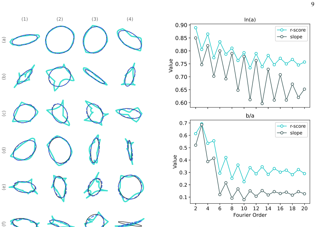
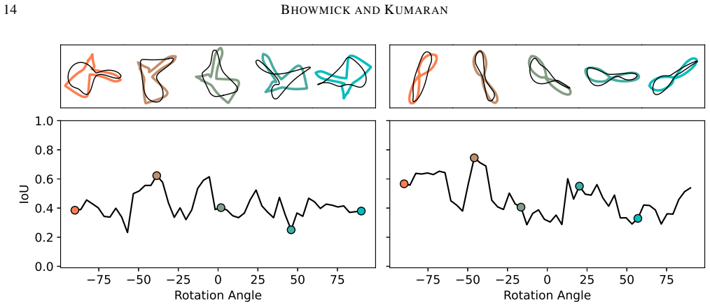
Shapes are decomposed into elliptical Fourier components that successively perturb an ideal ellipse; neural networks trained on the simulated light curves of these shapes recover the low-order coefficients that encode overall shape, orientation, and large-scale features, while higher-order coefficients allow scale recovery but limit inference of eccentricity and orientation, and non-convex features introduce orientation-dependent reconstruction errors.
What carries the argument
Fourier decomposition of a shape into a series of elliptical components that add diminishing perturbations to a base ellipse, with the neural network learning to map light curves back to those coefficients.
If this is right
- Low-order elliptical components that set overall shape, orientation, and large-scale perturbations can be reconstructed from light curves.
- Higher-order components permit reliable scale recovery but limit accurate inference of eccentricity and orientation.
- Reconstruction accuracy for non-convex features varies with the object's orientation relative to the line of sight.
- Transit light curves therefore contain usable geometric information beyond the spherical approximation.
Where Pith is reading between the lines
- Extending the training set to include three-dimensional projections and realistic noise levels would test whether the same network can handle actual telescope data.
- Because reconstruction of finer details depends on orientation, repeated transits at different viewing angles could supply additional constraints and improve higher-order recovery.
- The approach could be applied to known irregular solar-system objects observed in transit to provide an independent check on the method's limits.
Load-bearing premise
The library of simulated two-dimensional random shapes and their light curves is representative enough of real transiting objects and conditions to let the trained network generalize.
What would settle it
Take a transit light curve of a known irregular body such as a transiting asteroid whose three-dimensional shape has been measured independently, decompose that shape into the same Fourier elliptical components, and check whether the network's predicted low-order coefficients match the true values within the reported accuracy limits.
Figures


read the original abstract
Characterizing the geometry of an object orbiting around a star from its transit light curve is a powerful tool to uncover various complex phenomena. This problem is inherently ill-posed, since similar or identical light curves can be produced by multiple different shapes. In this study, we investigate the extent to which the features of a shape can be embedded in a transit light curve. We generate a library of two-dimensional random shapes and simulate their transit light curves with light curve simulator, Yuti. Each shape is decomposed into a series of elliptical components expressed in the form of Fourier coefficients that adds increasingly diminishing perturbations to an ideal ellipse. We train deep neural networks to predict these Fourier coefficients directly from simulated light curves. Our results demonstrate that the neural network can successfully reconstruct the low-order ellipses, which describe overall shape, orientation and large-scale perturbations. For higher order ellipses the scale is successfully determined but the inference of eccentricity and orientation is limited, demonstrating the extent of shape information in the light curve. We explore the impact of non-convex shape features in reconstruction, and show its dependence on shape orientation. The level of reconstruction achieved by the neural network underscores the utility of using light curves as a means to extract geometric information from transiting systems.
Editorial analysis
A structured set of objections, weighed in public.
Referee Report
Summary. The manuscript proposes training deep neural networks on simulated transit light curves of two-dimensional random shapes generated by the Yuti simulator. Each shape is decomposed into a Fourier series of elliptical components with diminishing perturbations. The central claim is that the network successfully recovers low-order Fourier coefficients describing overall shape, orientation, and large-scale perturbations, while higher-order coefficients allow scale recovery but show limited accuracy for eccentricity and orientation. The work concludes that this demonstrates the utility of light curves for extracting geometric information from transiting systems.
Significance. If the reconstruction holds under more realistic conditions, the approach could highlight the information content in transit photometry beyond spherical models, potentially aiding characterization of irregular or deformed transiting bodies. The Fourier ellipse decomposition provides a structured parameterization that could be extended, but current results are confined to idealized 2D simulations without key physical effects.
major comments (2)
- [§3] §3 (data generation and simulation): The library consists of purely two-dimensional shapes whose light curves are simulated without stellar limb darkening, three-dimensional orbital geometry (inclination, impact parameter), or photon noise. This assumption is load-bearing for the abstract's claim of utility for 'transiting systems,' as real observations are dominated by these effects; without them the reported reconstruction accuracy on clean simulations does not establish recoverability from observed data.
- [§4] §4 (results): The demonstration that 'the neural network can successfully reconstruct the low-order ellipses' is presented without quantitative metrics such as RMSE, correlation coefficients, error bars on test-set performance, validation splits, or ablation studies. This absence makes it impossible to assess the strength of the distinction between low- and high-order terms or to rule out overfitting.
minor comments (1)
- [Abstract] The abstract and introduction would benefit from explicit statements of the number of shapes in the training library, the maximum Fourier order considered, and the precise loss function used for training.
Simulated Author's Rebuttal
We thank the referee for their constructive and detailed feedback, which has helped us clarify the scope and strengthen the quantitative presentation of our results. We address each major comment point by point below.
read point-by-point responses
-
Referee: [§3] §3 (data generation and simulation): The library consists of purely two-dimensional shapes whose light curves are simulated without stellar limb darkening, three-dimensional orbital geometry (inclination, impact parameter), or photon noise. This assumption is load-bearing for the abstract's claim of utility for 'transiting systems,' as real observations are dominated by these effects; without them the reported reconstruction accuracy on clean simulations does not establish recoverability from observed data.
Authors: We agree that the simulations are idealized and omit limb darkening, three-dimensional orbital parameters, and photon noise. The study is designed as a controlled proof-of-concept to isolate the geometric information content in transit light curves. We have revised the abstract to temper the language regarding applicability to observed data and added a new paragraph in the Discussion section that explicitly lists these limitations and identifies incorporation of realistic effects as a priority for future work. revision: yes
-
Referee: [§4] §4 (results): The demonstration that 'the neural network can successfully reconstruct the low-order ellipses' is presented without quantitative metrics such as RMSE, correlation coefficients, error bars on test-set performance, validation splits, or ablation studies. This absence makes it impossible to assess the strength of the distinction between low- and high-order terms or to rule out overfitting.
Authors: We acknowledge the absence of explicit quantitative metrics in the original submission. In the revised manuscript we have added a table reporting RMSE and Pearson correlation coefficients for each Fourier coefficient on the test set, specified the train/validation/test split (70/15/15), included error bars derived from multiple random seeds, and incorporated an ablation study on network depth. These additions allow direct evaluation of the low- versus high-order performance difference and provide evidence against overfitting. revision: yes
Circularity Check
No significant circularity in simulation-to-prediction pipeline
full rationale
The paper generates a library of 2D random shapes, decomposes them into Fourier elliptical components, simulates transit light curves via the external Yuti simulator, and trains a neural network to map light curves back to those coefficients. This is a standard supervised learning setup on held-out simulated data with no evidence that the target Fourier coefficients are defined in terms of the network outputs, no fitted parameters renamed as predictions, and no load-bearing self-citations or uniqueness theorems. The central claim of successful low-order reconstruction is therefore independent of the inputs by construction and does not reduce to a tautology; any limitations on generalization to real 3D transits with limb darkening and noise are correctness concerns rather than circularity.
Axiom & Free-Parameter Ledger
axioms (2)
- domain assumption Transit light curves contain recoverable information about non-spherical shape features when shapes are expressed as sums of elliptical Fourier components.
- domain assumption The Yuti simulator produces light curves that are representative of real observations for the purpose of training.
Reference graph
Works this paper leans on
-
[1]
Abadi M., et al., 2015, TensorFlow : Large-Scale Machine Learning on Heterogeneous Systems, https://www.tensorflow.org/
work page 2015
-
[2]
Allworth J., Windrim L., Bennett J., Bryson M., 2021, @doi [Acta Astronautica] 10.1016/j.actaastro.2021.01.048 , https://ui.adsabs.harvard.edu/abs/2021AcAau.181..301A 181, 301
-
[3]
Barros S. C. C., et al., 2022, @doi [ ] 10.1051/0004-6361/202142196 , https://ui.adsabs.harvard.edu/abs/2022A&A...657A..52B 657, A52
-
[4]
Berardo D., de Wit J., 2022, @doi [ ] 10.3847/1538-4357/ac82b2 , https://ui.adsabs.harvard.edu/abs/2022ApJ...935..178B 935, 178
-
[5]
Bhowmick U., Khaire V., 2024, @doi [ ] 10.3847/1538-3881/ad7d8d , https://ui.adsabs.harvard.edu/abs/2024AJ....168..243B 168, 243
- [6]
-
[7]
Cellino A., Zappalà V., Farinella P., 1989, @doi [ ] https://doi.org/10.1016/0019-1035(89)90178-4 , https://ui.adsabs.harvard.edu/abs/1989Icar...78..298C 78, 298
-
[8]
Changeat Q., Ito Y., Al-Refaie A. F., Yip K. H., Lueftinger T., 2024, @doi [ ] 10.3847/1538-3881/ad3032 , https://ui.adsabs.harvard.edu/abs/2024AJ....167..195C 167, 195
-
[9]
pp 1 -- 4, @doi 10.1109/MMSP.2005.248668
Chen Y., Sundaram H., 2005, in IEEE 7th Workshop on Multimedia Signal Processing. pp 1 -- 4, @doi 10.1109/MMSP.2005.248668
-
[10]
Chen Z., Ji J., Chen G., Yan F., Tan X., 2025, @doi [ ] 10.3847/1538-3881/adc803 , https://ui.adsabs.harvard.edu/abs/2025AJ....169..294C 169, 294
-
[11]
Curry A., Booth R., Owen J. E., Mohanty S., 2024, @doi [ ] 10.1093/mnras/stae191 , https://ui.adsabs.harvard.edu/abs/2024MNRAS.528.4314C 528, 4314
-
[12]
E., 1943, Statistical Adjustment of Data
Deming W. E., 1943, Statistical Adjustment of Data. Wiley
work page 1943
-
[13]
https://amostech.com/2019-technical-papers/
Furfaro R., Linares R., Reddy V., 2019, in AMOS Technologies Conference, Maui Economic Development Board, Kihei, Maui, HI. https://amostech.com/2019-technical-papers/
work page 2019
-
[14]
Galeano D., Peltoniemi J., Enr \' quez-Caldera R., Guichard J., 2025, in Journal of Physics Conference Series. IOP, p. 012001, @doi 10.1088/1742-6596/2946/1/012001
-
[15]
Harmon R. O., Crews L. J., 2000, @doi [ ] 10.1086/316882 , https://ui.adsabs.harvard.edu/abs/2000AJ....120.3274H 120, 3274
-
[16]
Heller R., 2024, @doi [ ] 10.1051/0004-6361/202244087 , https://ui.adsabs.harvard.edu/abs/2024A&A...689A..97H 689, A97
-
[17]
Hornik K., Stinchcombe M., White H., 1989, @doi [Neural Networks] 10.1016/0893-6080(89)90020-8 , 2, 359
-
[18]
Jiang Y., Hu S., Du J., Chen X., Cao H., Liu S., Feng S., 2023, @doi [Aerospace] 10.3390/aerospace10010041 , https://www.mdpi.com/2226-4310/10/1/41 10, 41
-
[19]
Kaasalainen M., Torppa J., 2001, @doi [Icarus] https://doi.org/10.1006/icar.2001.6673 , https://ui.adsabs.harvard.edu/abs/2001Icar..153...24K 153, 24
-
[20]
Kaasalainen M., Torppa J., Muinonen K., 2001, @doi [Icarus] https://doi.org/10.1006/icar.2001.6674 , https://ui.adsabs.harvard.edu/abs/2001Icar..153...37K 153, 37
-
[21]
Kuhl F. P., Giardina C. R., 1982, @doi [Computer Graphics and Image Processing] https://doi.org/10.1016/0146-664X(82)90034-X , https://www.sciencedirect.com/science/article/pii/0146664X8290034X 18, 236
-
[22]
Lecavelier des Etangs A., et al., 2022, @doi [Scientific Reports] 10.1038/s41598-022-09021-2 , https://ui.adsabs.harvard.edu/abs/2022NatSR..12.5855L 12, 5855
-
[23]
Luger R., Foreman-Mackey D., Hedges C., Hogg D. W., 2021, @doi [ ] 10.3847/1538-3881/abfdb8 , https://ui.adsabs.harvard.edu/abs/2021AJ....162..123L 162, 123
-
[24]
Luo T., Liang Y., IP W.-H., 2019, @doi [ ] 10.3847/1538-3881/ab1b46 , https://ui.adsabs.harvard.edu/abs/2019AJ....157..238L 157, 238
-
[25]
Luo T., Liang Y.-Y., Ip W.-H., Huang H.-Z., Lin X.-X., 2021, @doi [Research in Astronomy and Astrophysics] 10.1088/1674-4527/21/4/89 , https://ui.adsabs.harvard.edu/abs/2021RAA....21...89L 21, 089
-
[26]
Muinonen K., Wilkman O., Cellino A., Wang X., Wang Y., 2015, @doi [Planetary and Space Science] https://doi.org/10.1016/j.pss.2015.09.005 , https://ui.adsabs.harvard.edu/abs/2015P&SS..118..227M 118, 227
-
[27]
Muinonen K., Torppa J., Wang X. B., Cellino A., Penttil \"a A., 2020, @doi [ ] 10.1051/0004-6361/202038036 , https://ui.adsabs.harvard.edu/abs/2020A&A...642A.138M 642, A138
-
[28]
Muinonen K., Uvarova E., Martikainen J., Penttilä A., Cellino A., Wang X., 2022, @doi [Frontiers in Astronomy and Space Sciences] 10.3389/fspas.2022.821125 , https://ui.adsabs.harvard.edu/abs/2022FrASS...9.1125M 9, 821125
-
[29]
Murphy M. M., et al., 2024a, @doi [Nature Astronomy] 10.1038/s41550-024-02367-9 , https://ui.adsabs.harvard.edu/abs/2024NatAs...8.1562M 8, 1562
-
[30]
Murphy M. M., Beatty T. G., Apai D., 2024b, @doi [ ] 10.3847/1538-4357/ad7114 , https://ui.adsabs.harvard.edu/abs/2024ApJ...974..179M 974, 179
-
[31]
Oliveira D. A. B., 2020, in IEEE 17th ISBI. pp 1798--1802, @doi 10.1109/ISBI45749.2020.9098676
-
[32]
Ostro S. J., Connelly R., Dorogi M., 1988, @doi [Icarus] https://doi.org/10.1016/0019-1035(88)90126-1 , https://www.sciencedirect.com/science/article/pii/0019103588901261 75, 30
-
[33]
Pedregosa F., et al., 2011, Journal of Machine Learning Research, https://ui.adsabs.harvard.edu/abs/2011JMLR...12.2825P 12, 2825
work page 2011
-
[34]
MIT Press, Cambridge, MA, pp 61--74, @doi 10.5555/645527.657447
Platt J., 1999, in , Advances in Large‑Margin Classifiers. MIT Press, Cambridge, MA, pp 61--74, @doi 10.5555/645527.657447
-
[35]
Roettenbacher R. M., Monnier J. D., Harmon R. O., Barclay T., Still M., 2013, @doi [ ] 10.1088/0004-637X/767/1/60 , https://ui.adsabs.harvard.edu/abs/2013ApJ...767...60R 767, 60
-
[36]
Santos A. R. G., Cunha M. S., Avelino P. P., Garc \' a R. A., Mathur S., 2017, @doi [ ] 10.1051/0004-6361/201629923 , https://ui.adsabs.harvard.edu/abs/2017A&A...599A...1S 599, A1
-
[37]
Saxena P., Panka P., Summers M., 2015, @doi [ ] 10.1093/mnras/stu2111 , https://ui.adsabs.harvard.edu/abs/2015MNRAS.446.4271S 446, 4271
-
[38]
Selhorst C. L., Barbosa C. L., Sim \ o es P. J. A., Vidotto A. A., Valio A., 2020, @doi [ ] 10.3847/1538-4357/ab89a4 , https://ui.adsabs.harvard.edu/abs/2020ApJ...895...62S 895, 62
-
[39]
Tang Y., Ying C., Xia C., Zhang X., Jiang X., 2025, @doi [ ] 10.1051/0004-6361/202452058 , https://ui.adsabs.harvard.edu/abs/2025A&A...696A..55T 696, A55
-
[40]
Viquerat J., Hachem E., 2020, @doi [Computers & Fluids] https://doi.org/10.1016/j.compfluid.2020.104645 , https://www.sciencedirect.com/science/article/pii/S0045793020302164 210, 104645
-
[41]
Viquerat J., Rabault J., Kuhnle A., Ghraieb H., Larcher A., Hachem E., 2021, @doi [Journal of Computational Physics] 10.1016/j.jcp.2020.110080 , https://sciencedirect.com/science/article/pii/S0021999120308548 428, 110080
-
[42]
Wang X., Nie Z., Gong J., Liang Z., 2021, @doi [Construction and Building Materials] https://doi.org/10.1016/j.conbuildmat.2020.121468 , https://www.sciencedirect.com/science/article/pii/S0950061820334723 268, 121468
-
[43]
Williams P. K. G., Charbonneau D., Cooper C. S., Showman A. P., Fortney J. J., 2006, @doi [ ] 10.1086/506468 , https://ui.adsabs.harvard.edu/abs/2006ApJ...649.1020W 649, 1020
-
[44]
Yip K. H., Tsiaras A., Waldmann I. P., Tinetti G., 2020, @doi [ ] 10.3847/1538-3881/abaabc , https://ui.adsabs.harvard.edu/abs/2020AJ....160...171Y 160, 171
-
[45]
Zhilkin A. G., Bisikalo D. V., 2020, @doi [Astronomy Reports] 10.1134/S1063772920080090 , https://ui.adsabs.harvard.edu/abs/2020ARep...64..563Z 64, 563
-
[46]
von Paris P., Gratier P., Bord \'e P., Leconte J., Selsis F., 2016, @doi [ ] 10.1051/0004-6361/201527894 , https://ui.adsabs.harvard.edu/abs/2016A&A...589A..52V 589, A52
discussion (0)
Sign in with ORCID, Apple, or X to comment. Anyone can read and Pith papers without signing in.