REVIEW 4 major objections 5 minor 6 cited by
A posterior that scores the averaged model, not the parameter, predicts better under misspecification.
Reviewed by Pith at T0; open to challenge. T0 means a machine referee read the full paper against a public rubric. the ladder, T0–T4 →
T0 review · deepseek-v4-flash
2026-08-04 12:46 UTC pith:JPHOF264
load-bearing objection Useful framework and sampler, but the dominance claims over classical Bayes don't follow from the theory as stated. the 4 major comments →
Predictively Oriented Posteriors
The pith
A machine-rendered reading of the paper's core claim, the machinery that carries it, and where it could break.
Core claim
The paper's central finding is that a posterior defined by scoring the predictive mixture rather than individual parameters is adaptively optimal for prediction. Formally, the PrO posterior is Qn = argmin_Q { λ_n ∫ L_n(θ_{1:k}) dQ^k + KL(Q||Π) }. Under convex scoring rules and sub-Gaussian loss conditions, Lemma 1 gives PAC-Bayes-type bounds, and Theorems 1 and 2 show that in well-specified settings the PrO predictive is within log(n)/√n of the Gibbs predictive, while under non-trivial misspecification it strictly dominates and approaches the predictively optimal mixture. If the model allows convex recovery of the data-generating distribution, the PrO predictive recovers it at rate log(n)/√n
What carries the argument
The key object is the predictive distribution P_Q = ∫ P_θ dQ(θ), with the scoring rule S applied to P_Q rather than to each P_θ. The paper uses a Jensen-type decomposition, S(P_Q, x) = ∫ S(P_θ, x)dQ - Δ(Q,x), and, under assumptions (DI) or (MS), represents the predictive score as an expectation over a product measure: ∫ L(θ_{1:k}, x)dQ^k(θ_{1:k}). This product-measure representation turns the PrO posterior into a KL-regularised expected-loss minimisation to which PAC-Bayes / Donsker-Varadhan arguments apply, yielding the key Lemma 1. For computation, the same objective is treated as a functional on the space of measures and minimised by a Wasserstein gradient flow, realised as a mean-field L
Load-bearing premise
The load-bearing premise is that the loss used to score predictions has Gaussian-like tail behaviour uniformly over all parameter combinations; if this concentration condition fails, the PAC-Bayes lemma and every rate or dominance result built on it can collapse.
What would settle it
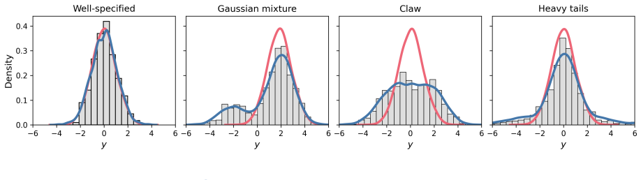
Simulate a large sample from a mixture such as P0 = 0.5 N(-2,1) + 0.5 N(2,1), fit a Gaussian location model with both the MMD-based PrO posterior and the Gibbs posterior, and compare their predictive divergences and posterior spread. If the PrO posterior collapses to a point mass, or if its predictive divergence fails to be strictly below the Gibbs predictive for large finite n, the adaptivity claim is falsified. More directly, check Assumption 3: for a Student-t likelihood with low degrees of freedom, compute the moment generating function; if the Hoeffding-type bound fails, the theory no lon
If this is right
- PrO posteriors give a principled way to combine prediction and uncertainty: the posterior remains a useful predictive mixture even when no single parameter value is true.
- They recover the predictively optimal model average at parametric rate (up to logs) when the predictive score is exact and tractable, and at n^{-1/3} for multi-sample log-score approximations.
- They concentrate around the true parameter in well-specified models, so the method does not sacrifice classical Bayesian consistency.
- They provide a quantitative notion of irreducible uncertainty due to misspecification: the non-degenerate limit can be interpreted as the degree of model misspecification.
- The particle sampling algorithm makes these posteriors computable for arbitrary convex scoring rules, not just special cases.
Where Pith is reading between the lines
- The paper leaves implicit a natural extension: the difference in spread between a PrO posterior and a Gibbs posterior could be turned into a formal misspecification test, since only the PrO posterior remains non-degenerate under non-trivial misspecification.
- If the adaptivity result is robust, PrO posteriors could serve as a principled replacement for cross-validated stacking in model averaging, with the posterior itself selecting the weights of the optimal predictive mixture.
- The theory assumes i.i.d. data; extending to dependent data is the obvious next stress test, and the particle dynamics may carry over, but the PAC-Bayes lemma would need mixing conditions.
- The choice of scoring rule becomes a modelling decision: different scores will produce different 'irreducible uncertainty' sets, offering a new way to compare model classes by their predictive geometry.
Editorial analysis
A structured set of objections, weighed in public.
Referee Report
Summary. The paper proposes 'predictively oriented' (PrO) posteriors, defined by minimizing a KL-regularized expected predictive scoring rule applied to the averaged predictive distribution P_Q = ∫ P_θ dQ(θ), rather than to individual parameters. The central claims are that PrO posteriors converge to the predictively optimal model average at rate n^{-1/2} up to log factors, predictively dominate classical and generalized Bayes posteriors, and adapt to model misspecification: they concentrate on the true parameter when the model is well-specified but remain non-degenerate under non-trivial misspecification. The theoretical core is a PAC-Bayes lemma (Lemma 1), followed by theorems for exact/tractable scores, DI-based approximations, and MS-based log-score approximations; computation is addressed via mean-field Langevin dynamics; several numerical illustrations are provided.
Significance. If the claims hold, PrO posteriors would be a valuable new inferential principle that combines parameter interpretability with predictive optimality and offers a principled resolution to posterior collapse under misspecification. The paper's strengths include a genuinely general PAC-Bayes bound (Lemma 1) that applies to exact and approximate predictive scores, detailed proofs in Section 7, and a plausible sampling algorithm via Wasserstein gradient flow. The MS-based log-score bound (Theorem 7) is an improvement over earlier vacuous bounds of Morningstar et al. (2022). However, the headline claims go substantially beyond what the theorems prove, and several statements need correction before the paper can be accepted.
major comments (4)
- [Abstract; §1.1; §7 (intro)] The abstract claims PrO posteriors 'predictively dominate both classical and generalised Bayes posterior predictive distributions.' But classical Bayes is defined in §1.1 as the Gibbs posterior with λ_n = n, while §7 states that all theoretical results use λ_n optimized with respect to Lemma 1, i.e. λ_n ∝ √(n/kC_k²) (or n^{1/3}/log n for MS log scores). Theorems 1, 3, and 4 therefore compare PrO posteriors only to Gibbs posteriors with this tuned, slower-growing λ_n, not to classical Bayes at λ_n = n. No theorem covers the λ_n = n regime. The empirical normal-location study in Appendix D.3 sets λ_n = n, which is outside the scope of the stated theorems.
- [§7.1.1, Theorem 3] Theorem 3 establishes E[D_S(P_{Q_n},P_0) − D_S(P_{Q†_n},P_0)] ≤ C log(n)/n^{1/2}. The prose then says 'the PrO posterior predictive performance is never worse than the Gibbs posterior.' This is not implied: the bound is a one-sided expected difference and permits E[D_S(P_{Q_n},P_0)] to exceed E[D_S(P_{Q†_n},P_0)] by up to O(log n/√n). The strict dominance in Theorem 4 requires Assumption 5 and the condition KL(Q̃⋆||Π)/λ_n + kλ_n C_k²/n ≤ JenGap/4. At λ_n = n this becomes KL(Q̃⋆||Π)/n + kC_k² ≤ JenGap/4, which fails whenever the misspecification gap JenGap is smaller than the fixed constant kC_k². Thus the classical-Bayes regime is again excluded.
- [Abstract; Lemma 1; Corollary 1; Theorem 7] The n^{-1/2} rate in the abstract is only proved for exact, tractable predictive scores with λ_n tuned to balance the PAC-Bayes terms in Lemma 1. At λ_n = n, the term λ_n kC_k²/n = kC_k² is O(1), so the bound does not vanish. For the logarithmic scoring rule, the only proved rate is n^{-1/3} (Corollary 1 and Theorem 7). The abstract's unqualified 'rate n^{-1/2}' and 'converge to the predictively optimal model average at rate n^{-1/2}' therefore overstate the theorem coverage. The claims should be qualified by score type, approximation, and the tuned λ_n regime.
- [Assumption 3; Assumption 10; §2.2] Assumption 3 requires a joint Hoeffding/sub-Gaussian condition on L(θ_{1:k},X), and the paper admits that for log scores this must be checked for each approximation. Theorem 7 uses the pointwise Assumption 10, which requires log p_θ(X) to be sub-Gaussian for every θ. For the standard Gaussian location model, log p_θ(X) is quadratic in X, and its exponential moment exists only for finitely many λ, so Assumption 10 fails. Thus the log-score theory does not cover one of the most natural motivating examples. The numerical evaluation of the normal-location model uses MMD and is covered, but the conceptual link to classical Bayes under the log score is not. This scope restriction should be stated prominently.
minor comments (5)
- [Lemma 1] The phrase 'if the scoring rule is exact so that bS=S, i.e., (3) holds' conflates exactness with tractability. The log score is exact for the predictive distribution but does not satisfy (3). The second part of Lemma 1 requires both bS=S and the tractability representation (3), and this should be stated explicitly.
- [§1.1 and throughout] Typographical: 'tenants' should be 'tenets' (e.g., 'follow the tenants of classical Bayesian analysis').
- [§4.3] The optimal λ_n suggestions in §4.3 are stated as if they are theorems. They follow from the calculations in Section 7, but no pointer is given to the precise result for exact/DI scores. A cross-reference would help.
- [References] The reference 'Chazal et al. (2025)' appears twice with slightly different author lists and venues; these should be merged. There is also a typo 'Corollay 1' in §4.3.
- [Appendix D.3] The normal-location experiments set λ_n = n, but Section 7 and §4.3 state that the theory uses λ_n ∝ √(n) (or slower). The authors should either add a theoretical justification for λ_n = n in these examples or re-run with the theoretically supported λ_n.
Circularity Check
No significant circularity: central PrO posterior guarantees are derived from the stated optimization objective via a PAC-Bayes bound, with independently defined comparison benchmarks.
full rationale
The paper's central derivation chain is self-contained rather than circular. The PrO posterior is defined as the minimizer of an empirical predictive-score objective plus KL regularization (equation (4)), and this definition does not presuppose the theorem conclusions. Lemma 1 is proved from Donsker–Varadhan and Assumption 3, yielding an upper bound on the expected predictive divergence in terms of an oracle infimum over Q plus KL and λ_n terms; the claimed n^{-1/2} rates then follow by explicitly optimizing λ_n with respect to that bound, not by fitting to test data or renaming an input. The oracle inf_Q D_S(P_Q, P_0) is a genuine benchmark: it is the population minimizer of the same divergence, not a parameter fitted to achieve the paper's claims. The strict dominance statements in Theorem 4 and related results rely on explicit assumptions such as non-trivial misspecification (Definition 2) and Assumption 5 (AppGap < misspecification gap), which are stated conditions rather than conclusions smuggled in by definition. Self-citations to the authors' prior work (e.g., Wild et al. 2023, Shen et al. 2025, McLatchie et al. 2025) provide algorithmic tools and existing convergence arguments, but the theorems establishing predictive rates and misspecification adaptivity do not reduce to those citations. The mismatch between the theoretical λ_n ∝ √n tuning and the λ_n = n used in some experiments is a scope/validity concern, not a circularity, and the same is true for the one-sided nature of Theorem 3's 'never worse' phrasing. No step was found in which a prediction is equivalent by construction to a fitted input or to a self-citation chain.
Axiom & Free-Parameter Ledger
free parameters (5)
- learning rate λ_n =
theory: ∝ √(n/k C_k²) ≈ n^{1/2}/log n; examples: n or n^{1/2}
- MS sample size k =
theory: ∝ (n/log n)^{1/3} for log score; examples: k=2
- kernel bandwidth for MMD =
median heuristic from the data (Appendix D.1)
- WGF step size dt =
varying values, 'chosen by visual inspection' (Appendix D.3)
- number of particles p and burn-in =
p = 10 to 64 depending on example; burn-in by eye
axioms (9)
- domain assumption Assumption 1: scoring rule S(P,x) is convex in P and the induced divergence D_S is jointly convex.
- domain assumption Assumption 2: predictive score can be represented as ∫ L(θ1:k,x)dQ^k and L satisfies (DI) or (MS).
- domain assumption Assumption 3: Hoeffding-type sub-Gaussianity of L(θ1:k,X): ∫ E[e^{λ(L−L_n)}] dΠ^k ≤ e^{λ²C_k²/n}.
- domain assumption Assumption 4: prior mass condition Π(B_r) ≥ (r/c_S)^{d_S} near the best parameter θ*.
- ad hoc to paper Assumption 5: AppGap(Q*,k) < D_S(P_θ*,P0) − D_S(P_Q*,P0).
- domain assumption Assumption 6: for any Q there exists Q̃ with finite KL and arbitrarily close loss.
- domain assumption Assumption 7: convex recovery holds via a continuous or discrete mixture with prior mass near components.
- ad hoc to paper Assumption 8: identifiability, metric compatibility, and reverse Hölder condition d2(PQ,PQ')^α ≤ D_S(PQ,PQ').
- domain assumption Assumptions 9-10: finite fourth moments of density ratios and pointwise sub-Gaussianity of log p_θ(X).
Cite this review
Pith. "Pith review of Predictively Oriented Posteriors." pith.science (2026). https://pith.science/paper/JPHOF264
@misc{pith2026251001915,
  author       = {Pith},
  title        = {Pith review of: Predictively Oriented Posteriors},
  year         = {2026},
  howpublished = {\url{https://pith.science/paper/JPHOF264}},
  note         = {Machine review of arXiv:2510.01915}
}
read the original abstract
We advocate for a new statistical principle that combines the most desirable aspects of both parameter inference and density estimation. This leads us to the predictively oriented (PrO) posterior, which expresses uncertainty as a consequence of predictive ability. We show that these posteriors converge to the predictively optimal model average and predictively dominate both classical and generalised Bayes posterior predictive distributions. Further, PrO posteriors adapt to the level of model misspecification: while they concentrate around the true model in the same way as classical and generalised Bayesian strategies if the model can recover the data-generating distribution, they do not concentrate around a single model in the presence of non-trivial forms of model misspecification. Instead, they stabilise towards a non-degenerate predictively optimal posterior distribution that represents a form of irreducible uncertainty due to model misspecification. We put forward a sampling algorithm for PrO posteriors based on mean field Langevin dynamics, and verify the practical significance of our theoretical developments on a number of numerical examples.
Figures


Forward citations
Cited by 6 Pith papers
-
Thinned Mean Field Langevin Dynamics
KT-MFLD thins the particle system in mean-field Langevin dynamics to O(N^{3/2}) complexity with convergence guarantees matching standard MFLD up to logarithmic factors.
-
Predictively-Oriented Kalman Filtering
EKF-PrO is a fast linear-Gaussian approximation to predictively-oriented posteriors for online filtering, with no tunable hyperparameters and cost comparable to standard methods.
-
Detecting Model Misspecification in Bayesian Inverse Problems via Variational Gradient Descent
Comparing the standard Bayesian posterior to a predictive-oriented mixture posterior Q fitted via variational gradient descent detects model misspecification in inverse problems.
-
Detecting Model Misspecification in Bayesian Inverse Problems via Variational Gradient Descent
Comparing the Bayesian predictive distribution to a predictively oriented mixture posterior — both computed with variational gradient descent — detects model misspecification.
-
Soft Specialists: $\alpha$-R\'enyi Ensembles for Uncertainty-Aware LLM Post-Training
An α-Rényi variational ensemble method learns distributions over LoRA adapter parameters for uncertainty-aware LLM post-training, balancing individual model plausibility with complementary specialization.
-
A Divergence-Based Method for Weighting and Averaging Model Predictions
A minimum divergence method for model weighting in prediction averaging shows small-sample advantages over stacking and Akaike-style weighting.
Reference graph
Works this paper leans on
-
[1]
Aitchison, J. (1975). Goodness of prediction fit. Biometrika\/ 62\/ (3), 547--554
1975
-
[2]
Alquier, P. (2024). User-friendly introduction to PAC - B ayes bounds. Foundations and Trends in Machine Learning\/ 17\/ (2), 174--303
2024
-
[3]
Alquier, P. and M. Gerber (2024, February). Universal robust regression via maximum mean discrepancy. Biometrika\/ 111\/ (1), 71--92. Publisher: Oxford University Press (OUP)
2024
-
[4]
Ridgway, and N
Alquier, P., J. Ridgway, and N. Chopin (2016). On the properties of variational approximations of G ibbs posteriors. The Journal of Machine Learning Research\/ 17\/ (1), 8374--8414
2016
-
[5]
Altamirano, M., F.-X. Briol, and J. Knoblauch (2023a). Robust and conjugate G aussian process regression. arXiv preprint arXiv:2311.00463\/
-
[6]
Briol, and J
Altamirano, M., F.-X. Briol, and J. Knoblauch (2023b). Robust and scalable B ayesian online changepoint detection. In International Conference on Machine Learning . PMLR
-
[7]
Audibert, J.-Y. (2004). Pac-bayesian statistical learning theory. These de doctorat de l’Universit \'e Paris\/ 6 , 29
2004
-
[8]
Dreassi, L
Berti, P., E. Dreassi, L. Pratelli, and P. Rigo (2021). A class of models for Bayesian predictive inference. Bernoulli\/ 27\/ (1), 702--726
2021
-
[9]
Bissiri, P. G., C. C. Holmes, and S. G. Walker (2016). A general framework for updating belief distributions. J. Royal Statist. Society Series B\/ 78\/ (5), 1103--1130
2016
-
[10]
(2001, August)
Breiman, L. (2001, August). Statistical Modeling : The Two Cultures (with comments and a rejoinder by the author). Statistical Science\/ 16\/ (3)
2001
-
[11]
Catoni, O. (2007). Pac-Bayesian Supervised Classification: The Thermodynamics of Statistical Learning , Volume 56. Institute of Mathematical Statistics
2007
-
[13]
Chazal, C., H. Kanagawa, Z. Shen, A. Korba, and C. J. Oates (2025, September). A Computable Measure of Suboptimality for Entropy - Regularised Variational Objectives . arXiv:2509.10393 [stat]
Pith/arXiv arXiv 2025
-
[14]
Ch \'e rief-Abdellatif, B.-E. and P. Alquier (2020). MMD - B ayes: Robust B ayesian estimation via maximum mean discrepancy. In Symposium on Advances in Approximate B ayesian Inference , pp.\ 1--21. PMLR
2020
-
[15]
Cherief-Abdellatif, B.-E., R. Douc, A. Doucet, and H. Marival (2025). On the asymptotics of importance weighted variational inference. arXiv preprint arXiv:2501.08477\/
Pith/arXiv arXiv 2025
-
[16]
Del Moral, P. (2013). Mean field simulation for monte carlo integration. Monographs on Statistics and Applied Probability\/ 126\/ (26), 6
2013
-
[17]
Altamirano, A
Duran-Martin, G., M. Altamirano, A. Shestopaloff, L. S \'a nchez-Betancourt, J. Knoblauch, M. Jones, F.-X. Briol, and K. P. Murphy (2024). Outlier-robust kalman filtering through generalised bayes. In International Conference on Machine Learning , pp.\ 12138--12171. PMLR
2024
-
[18]
Holmes, and S
Fong, E., C. Holmes, and S. G. Walker (2023). Martingale posterior distributions. Journal of the Royal Statistical Society Series B: Statistical Methodology\/ 85\/ (5), 1357--1391
2023
-
[19]
Fortini, S. and S. Petrone (2020). Quasi- Bayes Properties of a Procedure for Sequential Learning in Mixture Models . Journal of the Royal Statistical Society Series B: Statistical Methodology\/ 82\/ (4), 1087--1114
2020
-
[20]
Fortini, S. and S. Petrone (2023). Prediction-based uncertainty quantification for exchangeable sequences. Philosophical Transactions of the Royal Society A: Mathematical, Physical and Engineering Sciences\/ 381\/ (2247), 20220142
2023
-
[21]
Fortini, S. and S. Petrone (2025). Exchangeability, prediction and predictive modeling in Bayesian statistics. Statistical Science\/ 40\/ (1), 40--67
2025
-
[22]
Frazier, D. T., J. Knoblauch, J. Jewson, and C. Drovandi (2025). Exact sampling of gibbs measures with estimated losses. arXiv preprint arXiv:2404.15649\/
Pith/arXiv arXiv 2025
-
[23]
Iwata, I
Futami, F., T. Iwata, I. Sato, M. Sugiyama, et al. (2021). Loss function based second-order jensen inequality and its application to particle variational inference. Advances in Neural Information Processing Systems\/ 34 , 6803--6815
2021
-
[24]
Iwata, N
Futami, F., T. Iwata, N. Ueda, I. Sato, and M. Sugiyama (2022). Predictive variational bayesian inference as risk-seeking optimization. In International Conference on Artificial Intelligence and Statistics , pp.\ 5051--5083. PMLR
2022
-
[25]
Garreau, D., W. Jitkrittum, and M. Kanagawa (2018, October). Large sample analysis of the median heuristic. arXiv:1707.07269 [math]
Pith/arXiv arXiv 2018
-
[26]
Gelman, A. and D. Nolan (2002, September). A Probability Model for Golf Putting . Teaching Statistics\/ 24\/ (3), 93--95. Publisher: Wiley
2002
-
[27]
Germain, P., F. Bach, A. Lacoste, and S. Lacoste-Julien (2016). PAC - B ayesian theory meets B ayesian inference. Advances in Neural Information Processing Systems\/ 29
2016
-
[28]
Germain, P., A. Lacasse, F. Laviolette, M. Marchand, and J.-F. Roy (2015). Risk bounds for the majority vote: From a pac-bayesian analysis to a learning algorithm. arXiv preprint arXiv:1503.08329\/
Pith/arXiv arXiv 2015
-
[29]
Ghosal, S., J. K. Ghosh, and A. W. van der Vaart (2000). Convergence rates of posterior distributions. Ann. Statist.\/ 28\/ (2), 500--531
2000
-
[30]
Balabdaoui, and A
Gneiting, T., F. Balabdaoui, and A. E. Raftery (2007). Probabilistic forecasts, calibration and sharpness. Journal of the Royal Statistical Society: Series B (Statistical Methodology)\/ 69\/ (2), 243--268
2007
-
[31]
Gneiting, T. and A. E. Raftery (2007). Strictly proper scoring rules, prediction, and estimation. Journal of the American statistical Association\/ 102\/ (477), 359--378
2007
-
[32]
Gr \"u nwald, P. and T. van Ommen (2017). Inconsistency of bayesian inference for misspecified linear models, and a proposal for repairing it. Bayesian Analysis\/ 12\/ (4), 1069--1103
2017
-
[33]
Hauptvogel, N. and C. Igel (2024). On uniform, bayesian, and pac-bayesian deep ensembles. arXiv preprint arXiv:2406.05469\/
Pith/arXiv arXiv 2024
-
[34]
Horst, A. M., A. P. Hill, and K. B. Gorman (2020). palmerpenguins: Palmer Archipelago (Antarctica) penguin data . R package version 0.1.0
2020
-
[35]
Huber, P. (1964). Robust estimation of a location parameter. Ann. Statist.\/ 35 , 73--101
1964
-
[36]
Pleiss, and J
Jankowiak, M., G. Pleiss, and J. Gardner (2020a). Deep sigma point processes. In Proceedings of the 36th Conference on Uncertainty in Artificial Intelligence
-
[37]
Pleiss, and J
Jankowiak, M., G. Pleiss, and J. Gardner (2020b). Parametric G aussian process regressors. In Proceedings of the 37th International Conference on Machine Learning
-
[38]
Jiang, W. and M. A. Tanner (2008, October). Gibbs posterior for variable selection in high-dimensional classification and data mining. The Annals of Statistics\/ 36\/ (5)
2008
-
[39]
Kinderlehrer, and F
Jordan, R., D. Kinderlehrer, and F. Otto (1998). The variational formulation of the fokker--planck equation. SIAM journal on mathematical analysis\/ 29\/ (1), 1--17
1998
-
[40]
Jewson, and T
Knoblauch, J., J. Jewson, and T. Damoulas (2022). An optimization-centric view on B ayes' rule: Reviewing and generalizing variational inference. The Journal of Machine Learning Research\/ 23\/ (1), 5789--5897
2022
-
[41]
Knoblauch, J., J. E. Jewson, and T. Damoulas (2018). Doubly robust B ayesian inference for non-stationary streaming data with beta-divergences. Advances in Neural Information Processing Systems\/ 31
2018
-
[42]
Laviolette, M
Lacasse, A., F. Laviolette, M. Marchand, P. Germain, and N. Usunier (2006). Pac-bayes bounds for the risk of the majority vote and the variance of the gibbs classifier. Advances in Neural information processing systems\/ 19
2006
-
[43]
Lai, J. and Y. Yao (2024). Predictive variational inference: Learn the predictively optimal posterior distribution. arXiv preprint arXiv:2410.14843\/
Pith/arXiv arXiv 2024
-
[44]
Laird, N. (1978). Nonparametric maximum likelihood estimation of a mixing distribution. Journal of the American Statistical Association\/ 73\/ (364), 805--811
1978
-
[45]
Laplante, W., M. Altamirano, A. Duncan, J. Knoblauch, and F.-X. Briol (2025). Robust and conjugate spatio-temporal gaussian processes. arXiv preprint arXiv:2502.02450\/
Pith/arXiv arXiv 2025
-
[46]
Marchand, and J.-F
Laviolette, F., M. Marchand, and J.-F. Roy (2011). From pac-bayes bounds to quadratic programs for majority votes. In Proceedings of International Conference on Machine Learning , pp.\ 5--59
2011
-
[47]
Morvant, L
Laviolette, F., E. Morvant, L. Ralaivola, and J.-F. Roy (2017). Risk upper bounds for general ensemble methods with an application to multiclass classification. Neurocomputing\/ 219 , 15--25
2017
-
[48]
Leskel \"a , L. and M. Zhukov (2025). Sharp constants relating the sub-gaussian norm and the sub-gaussian parameter. arXiv preprint arXiv:2507.05928\/
Pith/arXiv arXiv 2025
-
[49]
Lindsay, B. G. (1995). Mixture models: theory, geometry, and applications. Ims
1995
-
[50]
Lorenzen, S. S., C. Igel, and Y. Seldin (2019). On pac-bayesian bounds for random forests. Machine Learning\/ 108\/ (8), 1503--1522
2019
-
[51]
Martin, R. and N. Syring (2022). Direct Gibbs posterior inference on risk minimizers: Construction , concentration, and calibration. In Handbook of Statistics , Volume 47, pp.\ 1--41. Elsevier
2022
-
[52]
Masegosa, A. (2020). Learning under model misspecification: Applications to variational and ensemble methods. Advances in Neural Information Processing Systems\/ 33 , 5479--5491
2020
-
[53]
Lorenzen, C
Masegosa, A., S. Lorenzen, C. Igel, and Y. Seldin (2020). Second order pac-bayesian bounds for the weighted majority vote. Advances in Neural Information Processing Systems\/ 33 , 5263--5273
2020
-
[54]
Knoblauch, F.-X
Matsubara, T., J. Knoblauch, F.-X. Briol, and C. J. Oates (2022). Robust generalised B ayesian inference for intractable likelihoods. Journal of the Royal Statistical Society Series B: Statistical Methodology\/ 84\/ (3), 997--1022
2022
-
[55]
Knoblauch, F.-X
Matsubara, T., J. Knoblauch, F.-X. Briol, and C. J. Oates (2023). Generalised B ayesian inference for discrete intractable likelihood. Journal of the American Statistical Association\/ (just-accepted), 1--21
2023
-
[56]
McLatchie, Y., E. Fong, D. T. Frazier, and J. Knoblauch (2025, July). Predictive performance of power posteriors. Biometrika\/ 112\/ (3), asaf034
2025
-
[57]
Miller, J. W. and D. B. Dunson (2019). Robust bayesian inference via coarsening. Journal of the American Statistical Association\/
2019
-
[58]
Morningstar, W. R., A. Alemi, and J. V. Dillon (2022). Pacm-bayes: Narrowing the empirical risk gap in the misspecified bayesian regime. In International Conference on Artificial Intelligence and Statistics , pp.\ 8270--8298. PMLR
2022
-
[59]
Ortega, L. A., R. Caba \ n as, and A. Masegosa (2022). Diversity and generalization in neural network ensembles. In International Conference on Artificial Intelligence and Statistics , pp.\ 11720--11743. PMLR
2022
-
[60]
Varoquaux, A
Pedregosa, F., G. Varoquaux, A. Gramfort, V. Michel, B. Thirion, O. Grisel, M. Blondel, P. Prettenhofer, R. Weiss, V. Dubourg, J. Vanderplas, A. Passos, D. Cournapeau, M. Brucher, M. Perrot, and E. Duchesnay (2011). Scikit-learn: Machine learning in P ython. Journal of Machine Learning Research\/ 12 , 2825--2830
2011
-
[61]
Pitas, K., H. A. Bourrous, and J. Arbel (2025). u -ensembles: Improved diversity in the small data regime using unlabeled data. In 7th Symposium on Advances in Approximate Bayesian Inference \ textendash \ Proceedings Track
2025
-
[62]
Robert, C. P. et al. (2007). The Bayesian choice: from decision-theoretic foundations to computational implementation , Volume 2. Springer
2007
-
[63]
Roberts, G. O. and J. S. Rosenthal (1998). Optimal scaling of discrete approximations to langevin diffusions. Journal of the Royal Statistical Society: Series B (Statistical Methodology)\/ 60\/ (1), 255--268
1998
-
[64]
Roberts, G. O. and R. L. Tweedie (1996). Exponential convergence of Langevin distributions and their discrete approximations . Bernoulli\/ 2\/ (4), 341 -- 363
1996
-
[65]
Schmon, S. M., P. W. Cannon, and J. Knoblauch (2020). Generalized posteriors in approximate bayesian computation. In Third Symposium on Advances in Approximate Bayesian Inference
2020
-
[66]
Knoblauch, S
Shen, Z., J. Knoblauch, S. Power, and C. J. Oates (2025). Prediction-centric uncertainty quantification via mmd. In The 28th International Conference on Artificial Intelligence and Statistics
2025
-
[67]
Sheth, R. and R. Khardon (2020). Pseudo- B ayesian learning via direct loss minimization with applications to sparse G aussian process models. In Proceedings of the 6th Symposium on Advances in Approximate Bayesian Inference
2020
-
[68]
Syring, N. and R. Martin (2019). Calibrating general posterior credible regions. Biometrika\/ 106\/ (2), 479--486
2019
-
[69]
Theisen, R., H. Kim, Y. Yang, L. Hodgkinson, and M. W. Mahoney (2024). When are ensembles really effective? Advances in neural information processing systems\/ 36 , 15015--15026
2024
-
[70]
van der Vaart, A. W. (1998). Asymptotic statistics , Volume 3. Cambridge: Cambridge University Press
1998
-
[71]
Van Der Vaart, A. W. and J. A. Wellner (1996). Weak convergence. In Weak convergence and empirical processes: with applications to statistics , pp.\ 16--28. Springer
1996
-
[72]
Germain, A
Viallard, P., P. Germain, A. Habrard, and E. Morvant (2021). Self-bounding majority vote learning algorithms by the direct minimization of a tight pac-bayesian c-bound. In Joint European Conference on Machine Learning and Knowledge Discovery in Databases , pp.\ 167--183. Springer
2021
-
[73]
Durand, and P
Vignault, L.-P., A. Durand, and P. Germain (2023). Erratum: Risk bounds for the majority vote: From a pac-bayesian analysis to a learning algorithm. Journal of Machine Learning Research\/ 24\/ (294), 1--13
2023
-
[74]
Wang, D. and Q. Liu (2019). Nonlinear stein variational gradient descent for learning diversified mixture models. In International Conference on Machine Learning , pp.\ 6576--6585. PMLR
2019
-
[75]
Sheth, and R
Wei, Y., R. Sheth, and R. Khardon (2021). Direct loss minimization for sparse gaussian processes. In International Conference on Artificial Intelligence and Statistics , pp.\ 2566--2574. PMLR
2021
-
[76]
Wild, V., J. Wu, D. Sejdinovic, and J. Knoblauch (2025). Near-optimal approximations for bayesian inference in function space. arXiv preprint arXiv:2502.18279\/
Pith/arXiv arXiv 2025
-
[77]
Wild, V. D., S. Ghalebikesabi, D. Sejdinovic, and J. Knoblauch (2023). A rigorous link between deep ensembles and (variational) bayesian methods. Advances in Neural Information Processing Systems\/ 36 , 39782--39811
2023
-
[78]
Masegosa, S
Wu, Y.-S., A. Masegosa, S. Lorenzen, C. Igel, and Y. Seldin (2021). Chebyshev-cantelli pac-bayes-bennett inequality for the weighted majority vote. Advances in Neural Information Processing Systems\/ 34 , 12625--12636
2021
-
[79]
Wu, Y.-S. and Y. Seldin (2022). Split-kl and pac-bayes-split-kl inequalities for ternary random variables. Advances in Neural Information Processing Systems\/ 35 , 11369--11381
2022
-
[80]
(1988, November)
Zellner, A. (1988, November). Optimal information processing and Bayes 's theorem. The American Statistician\/ 42\/ (4), 278
1988
-
[81]
(2006, October)
Zhang, T. (2006, October). From -entropy to KL -entropy: Analysis of minimum information complexity density estimation. The Annals of Statistics\/ 34\/ (5)
2006
discussion (0)
Sign in with ORCID, Apple, or X to comment. Anyone can read and Pith papers without signing in.