REVIEW 3 major objections 5 minor 44 references
The paper defines non-parametric probabilistic robustness (NPPR) as an infimum over all perturbation distributions within a budget, proves it lies between adversarial and fixed-distribution probabilistic robustness, and introduces a GMM-bas
Reviewed by Pith at T0; open to challenge. T0 means a machine referee read the full paper against a public rubric. the ladder, T0–T4 →
T0 review · deepseek-v4-flash
2026-08-03 20:55 UTC pith:DMY3PAK4
load-bearing objection The paper's headline metric collapses to adversarial robustness for any typical DNN, so the theory does not support the empirical claims—though the GMM estimator is a useful engineering contribution. the 3 major comments →
Non-Parametric Probabilistic Robustness: A Conservative Risk Estimator under Unknown Perturbation Distributions
The pith
A machine-rendered reading of the paper's core claim, the machinery that carries it, and where it could break.
Core claim
The central claim is that robustness evaluation need not commit to a noise model: for each input–label pair, NPPR is defined as the infimum, over all perturbation distributions supported within the budget, of the probability that the classifier's prediction remains unchanged. Proposition 1 establishes that this quantity sits between adversarial robustness (the deterministic worst case) and any fixed-distribution probabilistic robustness, so NPPR is a distribution-free conservative estimator. The accompanying estimator optimizes a GMM-based perturbation generator—conditioned on the input, the label, both, or neither—using a C&W-style margin loss as a surrogate for the hard indicator, and obta
What carries the argument
The central object is Definition 3's infimum over the admissible perturbation family P_epsilon, paired with a concrete estimator: MLP heads produce the GMM's mixture weights, means, and covariances (with dependency structures ranging from independent to fully input-and-label dependent), Gumbel–Softmax makes categorical sampling differentiable, a scaled tanh mapping keeps perturbations inside the L-infinity budget, and bicubic upsampling maps latent perturbations to image resolution. The C&W-style softplus margin loss relaxes the 0–1 indicator so the objective can be optimized by gradient descent.
Load-bearing premise
The load-bearing premise is that the GMM-plus-MLP estimator optimizes closely enough to the true infimum over all admissible perturbation distributions that its output remains a conservative estimate; the paper proves the inequality only for the exact infimum, not for the fitted approximation.
What would settle it
For a fixed image and perturbation budget, enumerate or search a dense family of candidate perturbation distributions (e.g., many Gaussian and mixture distributions with varied means/covariances inside the budget) and compute the model's correct-prediction rate under each. If any of these rates falls below the paper's NPPR estimate for that image, the estimator is not conservative and the Proposition 1 guarantee does not transfer to the estimate.
If this is right
- If NPPR is estimated faithfully, it provides a lower bound on robustness that holds regardless of the true (unknown) perturbation distribution.
- The inequality G_AR ≤ G_NPPR ≤ G_PR means that any PR evaluation based on a specified noise distribution can overestimate safety; NPPR corrects that by construction.
- Input- and label-dependent perturbation distributions yield lower NPPR than input-independent ones, so ignoring such dependencies understates risk.
- In the unrestricted distribution family, NPPR collapses to adversarial robustness, making NPPR a smooth bridge between average-case and worst-case robustness assessment.
- The estimator is practical on standard image benchmarks, producing up to roughly 40% more conservative PR estimates than fixed Gaussian or uniform baselines without requiring a predefined noise model.
Where Pith is reading between the lines
- The proof's equality case uses Dirac delta distributions, so the meaningful content of NPPR lies in the choice of the admissible family P_epsilon; the paper's GMM estimator restricts this family to mixtures, meaning its outputs are best read as practical upper bounds on the true NPPR rather than guaranteed lower bounds.
- The observed ordering—joint dependence giving the lowest NPPR, independence the highest—suggests a simple stress-testing recipe for deployment: use the joint-dependent estimator as the most pessimistic configuration when safety margins are tight.
- The same formulation could transfer to text, speech, or other modalities where distributional assumptions are even less settled, provided the perturbation generator can be reparameterized in that space.
- A fairer comparison of conservativeness would pit NPPR against a wide set of alternative learned distributions (e.g., adversarial-perturbation empirics or variational posteriors), not just fixed Gaussian/uniform noise.
Editorial analysis
A structured set of objections, weighed in public.
Referee Report
Summary. The paper introduces Non-Parametric Probabilistic Robustness (NPPR), defined as the infimum over all perturbation distributions supported in a norm ball of the expected correctness probability (Def. 3, Eq. 3). It claims theoretical inequalities among adversarial robustness (AR), probabilistic robustness (PR), and NPPR (Prop. 1), and proposes a GMM-based estimator with MLP heads and bicubic up-sampling (Sec. 4). Experiments on CIFAR-10/100 and Tiny ImageNet across several architectures report NPPR values intermediate between AR and PR, which the authors interpret as a more conservative, distribution-free robustness metric.
Significance. The paper identifies a legitimate limitation of existing PR formulations—their reliance on a fixed, known perturbation distribution—and proposes a natural response: optimize the distribution to obtain a conservative estimate. The experimental pipeline is extensive, and the distribution visualizations (Fig. 5) are informative. However, the formal metric as defined collapses to AR for any classifier with continuous decision regions: the infimum in Def. 3 is attained (or approached) by distributions supported on adversarial regions, making NPPR equal to AR. The proposed estimator minimizes a surrogate loss over a restricted GMM family, and no result guarantees that its value is a conservative estimate of the defined infimum. Consequently, the central claim that NPPR is a meaningful intermediate metric is not supported by the theory or the experiments.
major comments (3)
- [Sec. 3, Def. 3 and Prop. 1 (Eqs. 3, 6–7)] The infimum in Def. 3 over all distributions supported in B collapses to AR. For a classifier with continuous logits, if an adversarial perturbation exists in the interior of B, the set of adversarial perturbations contains an open neighborhood, which has positive Lebesgue measure. A continuous distribution supported on a small ball inside that neighborhood gives expected correctness 0, so S_NPPR(x,y)=S_AR(x,y) whenever an adversarial example exists. The strict-inequality branch in Eq. (7) assumes the adversarial set has measure zero, which is false for the open adversarial regions of real DNNs. Thus NPPR is not an intermediate metric; it is AR in disguise. The empirical values in Table 3 (e.g., 88.32% NPPR vs. 9.27% AR for ResNet18/CIFAR-10) therefore cannot be estimates of the Def. 3 infimum.
- [Sec. 4, Eqs. (9)–(11) and Table 3] The estimator minimizes a C&W softplus surrogate over a GMM parameterization, which is a strict subset of P_ε, and no bound relates the surrogate objective to the 0–1 indicator or the GMM family to the full P_ε. Since the GMM family is a subset of P_ε, the true NPPR is ≤ the obtained GMM value; the GMM value is an upper bound on the true NPPR, not a conservative lower estimate. The large gap between reported NPPR and AR (Table 3) is consistent with the estimator not approximating Def. 3 at all. A consistency or approximation theorem is needed but absent.
- [Appendix 7, Proof of Prop. 1 (Eqs. 23–35)] The proof of the unconditional-case reverse inequality is flawed. In Eqs. (33)–(35), the authors lower-bound E_ω[E_D[...]] by inf_ε E_D[...], but G_AR in the unconditional case is defined as inf_ε E_D[...] only in Prop. 2 (Eq. 40); in Prop. 1, G_AR is not this quantity. The definitions are inconsistent. Moreover, the proof of strict inequality (Eq. 25) asserts that if adversarial examples have measure zero under all continuous distributions, then all continuous ω yield expectation 1; this is false when the adversarial set has positive Lebesgue measure (which it does for DNNs). The theoretical chain G_AR < G_NPPR < G_PR is therefore not established for real classifiers.
minor comments (5)
- [Title / Abstract] The term 'non-parametric' is misleading since the proposed estimator is a Gaussian Mixture Model, a parametric family. The paper should clarify the distinction or qualify the term.
- [Sec. 5.3, Table 3] For WRN50 on CIFAR-10, the standard deviation for bGPR_Uniform is reported as 30.91, which is implausibly large compared to neighboring entries and likely a typographical error. Please verify.
- [Appendix 7, Proof 1] Typographical errors: 'exsit' should be 'exist'; Eq. (17) and surrounding text should consistently use the indicator 1_{h(x+ε)=y} rather than switching between correctness and error indicators.
- [Sec. 4, Eq. (11)] The softplus formulation is described as 'lower-bounds the loss at zero'; consider clarifying the sign convention, as the margin term is typically negative for adversarial examples.
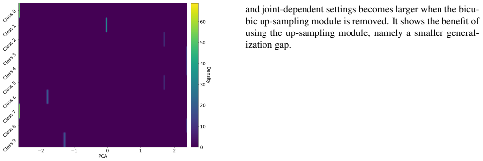
- [Sec. 5.1, Fig. 5] The caption mentions 'training dynamics of the NPPR' but it is unclear whether the plotted curve is the surrogate loss or the estimated 0–1 value. Please specify.
Circularity Check
The defined NPPR infimum equals AR by the paper's own Prop. 1 (Eq. 6), and the reported conservative estimates are the fitted GMM training objective — the middle-metric claim and its validation reduce to the definition and the fit.
specific steps
-
self definitional
[Def. 3 (Eq. 3); Prop. 1 (Eqs. 5–7); Appendix Sec. 7, Proof 1]
"Definition 3: ... S_NPPR(x,y) ≜ inf_{ω∈P_ε} E_{ε∼ω(·|x)}[1_{h(x+ε)=y}], where P_ε is the distribution family with support all lying within the perturbation budget B. Proposition 1: If we allow P_ε to be unrestricted, representing any family of distributions (including the Dirac delta measure), then the equality holds, G_AR = G_NPPR."
Def. 3 imposes no restriction on P_ε beyond support in B, so Dirac measures are in the family. The paper's own Prop. 1 (Eq. 6) then makes G_NPPR = G_AR the default value of the definition, not an 'extreme' case. The strict-inequality branch (Eq. 7) that would make NPPR a distinct middle metric requires both excluding Dirac measures and the adversarial set having measure zero in B; neither condition is in Def. 3, and for continuous classifiers any nonempty adversarial set is open (positive measure), so even continuous-only P_ε gives expected correctness 0 at any adversarial point. The exact metric therefore carries no content beyond AR; the reported bG_NPPR ≈ 88% vs bG_AR ≈ 9% (Table 3) cannot be estimates of this infimum.
-
fitted input called prediction
[Sec. 4, Eqs. (9)–(11); Sec. 5.3, Table 3]
"L(ϕ) = E_{(x,y)∼D}[E_{ε∼GMM_ϕ}[φ(h(x+U(ε)), y)]] (9) ... Our objective function can be interpreted as a global NPPR estimator that relaxes the hard 0–1 loss and models the perturbation distribution via a GMM."
The estimator is trained by minimizing Eq. (9)–(10), the empirical surrogate (softplus C&W margin, Eq. 11) of exactly the correctness probability later reported as bG_NPPR; the paper itself calls this objective 'a global NPPR estimator.' No theorem bounds the gap between the GMM-restricted surrogate optimum and the Def. 3 infimum over all of P_ε — Prop. 1 is proved only for the exact infimum. Hence the 'conservative (lower) PR estimates' in Table 3 are the fitted objective values of a restricted adversarial search (K=7 modes, 128-dim latent, bicubic up-sampling; the appendix admits the excluded input-space variant 'has a better performance'). The lower-than-PR prediction is forced by the training minimization, so the claimed confirmation of Prop. 1 (Sec. 5.3) reports the optimizer's output
full rationale
Def. 3 defines S_NPPR as the infimum over P_ε, 'the distribution family with support all lying within the perturbation budget B,' with no further restriction. The paper's own Prop. 1 (Eq. 6) then proves G_NPPR = G_AR once Dirac measures are admitted — and they are admitted by Def. 3 as written. The strict-inequality branch (Eq. 7) that would make NPPR a distinct middle metric requires both excluding Dirac measures from P_ε and the adversarial set having measure zero in B. Neither condition appears in Def. 3, and for the evaluated continuous ReLU classifiers any nonempty adversarial set is open with positive measure, so condition (ii) fails; restricting to continuous distributions does not restore a middle metric because a continuous distribution on a small ball inside an open adversarial region drives expected correctness to 0. Consequently the exact NPPR is AR (about 9%–4% in Table 3), not the reported 60%–98%: the numbers in Tables 1–3 are values of the fitted GMM/surrogate optimization of Sec. 4. That optimization minimizes the same correctness objective (Eqs. 9–11) that is later reported as the estimate, with no bound relating the GMM-restricted surrogate minimizer to the Def. 3 infimum; the paper explicitly says the objective 'can be interpreted as a global NPPR estimator.' Thus the 'conservative, lower' estimates are the fitted values of a restricted adversarial search, and the claim that experiments 'confirm Prop. 1' (Sec. 5.3) is the training outcome rather than an independent validation. Self-citations ([35]–[39], with overlapping authors) are numerous but not load-bearing for the derivation; the circularity here is definitional and estimation-based, not a self-citation chain.
Axiom & Free-Parameter Ledger
free parameters (6)
- GMM parameters (π_k, μ_k, Σ_k) =
learned by Adam on Eq. (10)
- Mixture components K =
3, 7, 12 (ablated)
- Latent perturbation dimension =
128 or 256
- Surrogate margin κ =
1
- Gumbel/annealing temperatures =
Tπ: 3→1, Tμ: 3→1, Tσ: 1.5→1, Gumbel: 1→0.1
- Learning rate / epochs =
5e-4 or 2e-2, 50 epochs
axioms (6)
- standard math GMMs can approximate any continuous distribution given enough components (Bishop 2006)
- standard math Gumbel-Softmax is a differentiable approximation to categorical sampling
- domain assumption Support of perturbation distributions is contained in the L∞ ball B via g_B = γ tanh(·)
- domain assumption For strict inequality G_AR < G_NPPR, adversarial perturbations form a measure-zero set under continuous distributions
- ad hoc to paper The surrogate C&W softplus margin loss is a faithful proxy for the 0/1 indicator
- domain assumption The four dependency structures cover the relevant perturbation scenarios
read the original abstract
Deep learning (DL) models, despite their remarkable success, remain vulnerable to small input perturbations that can cause erroneous outputs, motivating the recent proposal of probabilistic robustness (PR) as a complementary alternative to adversarial robustness (AR). However, existing PR formulations assume a fixed and known perturbation distribution, an unrealistic expectation in practice. To address this limitation, we propose non-parametric probabilistic robustness (NPPR), a more practical PR metric that does not rely on any predefined perturbation distribution. Following the non-parametric paradigm in statistical modeling, NPPR learns an optimized perturbation distribution directly from data, enabling conservative PR evaluation under distributional uncertainty. We further develop an NPPR estimator based on a Gaussian Mixture Model (GMM), covering various input-dependent and input-independent perturbation scenarios. Theoretical analyses establish the relationships among AR, PR, and NPPR. Extensive experiments on CIFAR-10, CIFAR-100, and Tiny ImageNet across ResNet18/50, WideResNet50 and VGG16 validate NPPR as a more practical robustness metric, showing conservative (lower) PR estimates compared to assuming those common perturbation distributions used in state-of-the-arts.
Figures


Reference graph
Works this paper leans on
-
[1]
Scalable quantitative verification for deep neural networks
Teodora Baluta, Zheng Leong Chua, Kuldeep S Meel, and Prateek Saxena. Scalable quantitative verification for deep neural networks. InICSE’21, pages 312–323, 2021. 1, 2
2021
-
[2]
Springer, 2006
Christopher M Bishop and Nasser M Nasrabadi.Pattern recognition and machine learning. Springer, 2006. 7
2006
-
[3]
Towards evaluating the robustness of neural networks
Nicholas Carlini and David Wagner. Towards evaluating the robustness of neural networks. InIEEE symposium on secu- rity and privacy (sp), pages 39–57, 2017. 3
2017
-
[4]
A survey on adversarial attacks and defences.CAAI Transactions on In- telligence Technology, 6(1):25–45, 2021
Anirban Chakraborty, Manaar Alam, Vishal Dey, Anupam Chattopadhyay, and Debdeep Mukhopadhyay. A survey on adversarial attacks and defences.CAAI Transactions on In- telligence Technology, 6(1):25–45, 2021. 1
2021
-
[5]
Universal adversarial perturbations: A survey.arXiv preprint arXiv:2005.08087,
Ashutosh Chaubey, Nikhil Agrawal, Kavya Barnwal, Keerat K Guliani, and Pramod Mehta. Universal adversarial perturbations: A survey.arXiv preprint arXiv:2005.08087,
Pith/arXiv arXiv 2005
-
[6]
Towards evaluating the robustness of neural networks learned by transduction
Jiefeng Chen, Xi Wu, Yang Guo, Yingyu Liang, and Somesh Jha. Towards evaluating the robustness of neural networks learned by transduction. InInternational Conference on Learning Representations, 2022. 7, 3
2022
-
[7]
Probabilistic robustness estimates for feed-forward neural networks.Neural networks, 142:138– 147, 2021
Nicolas Couellan. Probabilistic robustness estimates for feed-forward neural networks.Neural networks, 142:138– 147, 2021. 1, 2
2021
-
[8]
On the (non-) robustness of two-layer neural networks in different learning regimes
Elvis Dohmatob and Alberto Bietti. On the (non-) robustness of two-layer neural networks in different learning regimes. arXiv preprint arXiv:2203.11864, 2022. 2
Pith/arXiv arXiv 2022
-
[9]
Learning a deep convolutional network for image super-resolution
Chao Dong, Chen Change Loy, Kaiming He, and Xiaoou Tang. Learning a deep convolutional network for image super-resolution. InEuropean conference on computer vi- sion, pages 184–199. Springer, 2014. 2
2014
-
[10]
Acceler- ating the super-resolution convolutional neural network
Chao Dong, Chen Change Loy, and Xiaoou Tang. Acceler- ating the super-resolution convolutional neural network. In European conference on computer vision, pages 391–407. Springer, 2016. 7, 3
2016
-
[11]
Explaining and harnessing adversarial examples
Ian J Goodfellow. Explaining and harnessing adversarial examples. InInternational Conference on Learning Repre- sentations ICLR 2015. International Conference on Learning Representations, 2015. 1
2015
-
[12]
Safari: Versatile and efficient evaluations for robustness of interpretability
Wei Huang, Xingyu Zhao, Gaojie Jin, and Xiaowei Huang. Safari: Versatile and efficient evaluations for robustness of interpretability. InIEEE/CVF International Conference on Computer Vision (ICCV’23), pages 1988–1998, 2023. 4
1988
-
[13]
A survey of safety and trustworthiness of deep neural net- works: Verification, testing, adversarial attack and defence, and interpretability.Computer Science Review, 37:100270,
Xiaowei Huang, Daniel Kroening, Wenjie Ruan, and et al. A survey of safety and trustworthiness of deep neural net- works: Verification, testing, adversarial attack and defence, and interpretability.Computer Science Review, 37:100270,
-
[14]
Black-box adversarial at- tack with transferable model-based embedding
Zhichao Huang and Tong Zhang. Black-box adversarial at- tack with transferable model-based embedding. InInterna- tional Conference on Learning Representations, 2020. 7, 3
2020
-
[15]
Categorical reparameterization with gumbel-softmax.arXiv preprint arXiv:1611.01144, 2016
Eric Jang, Shixiang Gu, and Ben Poole. Categorical reparameterization with gumbel-softmax.arXiv preprint arXiv:1611.01144, 2016. 7, 3
Pith/arXiv arXiv 2016
-
[16]
Estimation of parti- cle transmission by random sampling.National Bureau of Standards applied mathematics series, 12:27–30, 1951
Herman Kahn and Theodore E Harris. Estimation of parti- cle transmission by random sampling.National Bureau of Standards applied mathematics series, 12:27–30, 1951. 4
1951
-
[17]
Cubic convolution interpolation for digital im- age processing.IEEE transactions on acoustics, speech, and signal processing, 29(6):1153–1160, 2003
Robert Keys. Cubic convolution interpolation for digital im- age processing.IEEE transactions on acoustics, speech, and signal processing, 29(6):1153–1160, 2003. 7, 3
2003
-
[18]
Chris J Maddison, Andriy Mnih, and Yee Whye Teh. The concrete distribution: A continuous relaxation of discrete random variables.arXiv preprint arXiv:1611.00712, 2016. 7, 3
Pith/arXiv arXiv 2016
-
[19]
John Wiley & Sons, 2000
Geoffrey J McLachlan and David Peel.Finite mixture mod- els. John Wiley & Sons, 2000. 7
2000
-
[20]
Adversarial robustness of deep neural networks: A survey from a formal verification perspective.IEEE Transactions on Dependable and Secure Computing, 2022
Mark Huasong Meng, Guangdong Bai, Sin Gee Teo, Zhe Hou, Yan Xiao, Yun Lin, and Jin Song Dong. Adversarial robustness of deep neural networks: A survey from a formal verification perspective.IEEE Transactions on Dependable and Secure Computing, 2022. 1
2022
-
[21]
The limitations of deep learning in adversarial settings
Nicolas Papernot, Patrick McDaniel, Somesh Jha, Matt Fredrikson, Z Berkay Celik, and Ananthram Swami. The limitations of deep learning in adversarial settings. InIEEE European symposium on security and privacy (EuroS&P), pages 372–387. IEEE, 2016. 1
2016
-
[22]
Cc-cert: A probabilistic approach to certify general robust- ness of neural networks
Mikhail Pautov, Nurislam Tursynbek, Marina Munkhoeva, Nikita Muravev, Aleksandr Petiushko, and Ivan Oseledets. Cc-cert: A probabilistic approach to certify general robust- ness of neural networks. InAAAI’22, pages 7975–7983,
-
[23]
Probabilistically robust learning: Balancing average and worst-case performance
Alexander Robey, Luiz Chamon, George J Pappas, and Hamed Hassani. Probabilistically robust learning: Balancing average and worst-case performance. InInternational Con- ference on Machine Learning, pages 18667–18686. PMLR,
-
[24]
In- triguing properties of neural networks
Christian Szegedy, Wojciech Zaremba, Ilya Sutskever, Joan Bruna, Dumitru Erhan, Ian Goodfellow, and Rob Fergus. In- triguing properties of neural networks. InIn Proc. of 2nd Int. Conf. on Learning Representations, 2014. 1
2014
-
[25]
Efficient sta- tistical assessment of neural network corruption robustness
Karim Tit, Teddy Furon, and Mathias Rousset. Efficient sta- tistical assessment of neural network corruption robustness. NeurIPS’21, 34:9253–9263, 2021. 1, 2
2021
-
[26]
Gradient- informed neural network statistical robustness estimation
Karim TIT, Teddy Furon, and Mathias Rousset. Gradient- informed neural network statistical robustness estimation. In Proc. of The 26th Int. Conf. on Artificial Intelligence and Statistics, pages 323–334. PMLR, 2023. 1, 2, 4
2023
-
[27]
Statistical analysis of finite mixture distributions
David Michael Titterington, Adrian FM Smith, and Udi E Makov. Statistical analysis of finite mixture distributions. (No Title), 1985. 7
1985
-
[28]
Statistically robust neural network classification
Benjie Wang, Stefan Webb, and Tom Rainforth. Statistically robust neural network classification. InUncertainty in Ar- tificial Intelligence, pages 1735–1745. PMLR, 2021. 1, 2, 4
2021
-
[29]
Real-esrgan: Training real-world blind super-resolution with pure synthetic data
Xintao Wang, Liangbin Xie, Chao Dong, and Ying Shan. Real-esrgan: Training real-world blind super-resolution with pure synthetic data. InProceedings of the IEEE/CVF inter- national conference on computer vision, pages 1905–1914,
1905
-
[30]
Zheng Wang, Geyong Min, and Wenjie Ruan. The implicit bias of gradient descent toward collaboration between lay- ers: A dynamic analysis of multilayer perceptions.Advances in Neural Information Processing Systems, 37:74868–74898,
-
[31]
A statistical approach to assessing neural network robustness
Stefan Webb, Tom Rainforth, Yee Whye Teh, and M Pawan Kumar. A statistical approach to assessing neural network robustness. InInt. Conf. on Learning Representations, 2019. 1, 2, 3, 4
2019
-
[32]
Proven: Verifying robustness of neural networks with a probabilistic approach
Lily Weng, Pin-Yu Chen, Lam Nguyen, Mark Squillante, Akhilan Boopathy, Ivan Oseledets, and Luca Daniel. Proven: Verifying robustness of neural networks with a probabilistic approach. InInt. Conf. on Machine Learning, pages 6727–
-
[33]
Fieldsend
Tianle Zhang, Wenjie Ruan, and Jonathan E. Fieldsend. Proa: A probabilistic robustness assessment against func- tional perturbations. InMachine Learning and Knowl- edge Discovery in Databases: European Conference, ECML PKDD 2022, Grenoble, France, September 19–23, 2022, Proceedings, Part III, page 154–170. Springer-Verlag, 2023. 1, 2, 3, 4
2022
-
[34]
Prass: probabilistic risk-averse robust learning with stochastic search
Tianle Zhang, Yanghao Zhang, Ronghui Mu, Jiaxu Liu, Jonathan Fieldsend, and Wenjie Ruan. Prass: probabilistic risk-averse robust learning with stochastic search. InPro- ceedings of the Thirty-Third International Joint Conference on Artificial Intelligence, pages 559–567, 2024. 2, 4
2024
-
[35]
Protip: Probabilistic robustness verification on text-to-image diffu- sion models against stochastic perturbation
Yi Zhang, Yun Tang, Wenjie Ruan, Xiaowei Huang, Sid- dartha Khastgir, Paul Jennings, and Xingyu Zhao. Protip: Probabilistic robustness verification on text-to-image diffu- sion models against stochastic perturbation. InEuropean Conference on Computer Vision, 2024. 1, 2, 3, 4
2024
-
[36]
Adversar- ial training for probabilistic robustness
Yi Zhang, Yuhang Chen, Zhen Chen, Wenjie Ruan, Xiaowei Huang, Siddartha Khastgir, and Xingyu Zhao. Adversar- ial training for probabilistic robustness. InProceedings of the IEEE/CVF International Conference on Computer Vision (ICCV), pages 1675–1685, 2025. 1
2025
-
[37]
Adversarial training for probabilistic robustness
Yi Zhang, Yuhang Chen, Zhen Chen, Wenjie Ruan, Xiaowei Huang, Siddartha Khastgir, and Xingyu Zhao. Adversarial training for probabilistic robustness. InProceedings of the IEEE/CVF International Conference on Computer Vision, pages 1675–1685, 2025. 2, 4
2025
-
[38]
Probabilistic robustness for free? revisiting training via a benchmark, 2025
Yi Zhang, Zheng Wang, Chen Zhen, Wenjie Ruan, Qing Guo, Siddartha Khastgir, Carsten Maple, and Xingyu Zhao. Probabilistic robustness for free? revisiting training via a benchmark, 2025. 1, 2, 4
2025
-
[39]
Probabilistic robustness in deep learning: A concise yet comprehensive guide.Adversarial Example De- tection and Mitigation Using Machine Learning, pages 1–13,
Xingyu Zhao. Probabilistic robustness in deep learning: A concise yet comprehensive guide.Adversarial Example De- tection and Mitigation Using Machine Learning, pages 1–13,
-
[40]
Adversar- ial robustness of neural networks from the perspective of lip- schitz calculus: A survey.ACM Computing Surveys, 2024
Monty-Maximilian Z ¨uhlke and Daniel Kudenko. Adversar- ial robustness of neural networks from the perspective of lip- schitz calculus: A survey.ACM Computing Surveys, 2024. 1, 2 Non-Parametric Probabilistic Robustness: A Conservative Metric with Optimized Perturbation Distributions Supplementary Material
2024
-
[41]
Proposition 3Considering AR, PR, and NPPR as defined in Def
Omitted Proofs To facilitate readability, we restate Propositions 1 and 2, fol- lowed by their proofs in order. Proposition 3Considering AR, PR, and NPPR as defined in Def. 1, 2, and 3, and binary loss function for AR, letGAR, GPR, andG NPPR denote their corresponding global robust- ness metrics. Given a perturbation distributionω∈P ε (either conditional ...
-
[42]
This quadratic growth ren- ders both storage and computation infeasible when the in- put dimension is large, as in modern image datasets
Details on Bicubic Up-sampling Since input images typically reside in high-dimensional spaces, the covariance matrix of the perturbation distribu- tion becomes prohibitively large, scaling asO(d 2)with re- spect to the input dimensiond. This quadratic growth ren- ders both storage and computation infeasible when the in- put dimension is large, as in moder...
-
[43]
one-hot,
Detailed Experiment Settings We provide the detailed experimental configurations in Tab. 4. For the independent–perturbation setting with a fixed up-sampler, we adopt a different training strategy from the other cases because this setting is substantially harder to optimize. Specifically, we use a larger learning rate of 2×10 −2 with a cosine cyclical sch...
-
[44]
Additional Experiments Here, we provide additional results that further illustrate the characteristics of the learned perturbation distributions. Fig. 6 presents the t-SNE visualization corresponding to Fig. 5 panel (d), but using the joint-dependence structure instead of label dependence. As shown, perturbation sam- ples from all classes become clearly d...
discussion (0)
Sign in with ORCID, Apple, or X to comment. Anyone can read and Pith papers without signing in.