REVIEW 4 major objections 6 minor 2 cited by
A network's learnable lag horizon is governed by the decay geometry of an effective learning rate envelope interacting with heavy-tailed gradient noise, producing logarithmic, polynomial, and exponential scaling regimes.
Reviewed by Pith at T0; open to challenge. T0 means a machine referee read the full paper against a public rubric. the ladder, T0–T4 →
T0 review · deepseek-v4-flash
2026-08-03 18:18 UTC pith:X4ONX5UF
load-bearing objection The learnability-window framework is a real idea, but the central mean-factorization step (Eq. 31) is unproven, the monotonicity lemma is not proved as written, and the experiments confirm the framework's own threshold. the 4 major comments →
Learnability Window in Gated Recurrent Neural Networks
The pith
A machine-rendered reading of the paper's core claim, the machinery that carries it, and where it could break.
Core claim
The paper's central claim is that numerical stability of state-transition Jacobian products is not sufficient for temporal learnability; instead, learnability is determined by whether the effective learning rate envelope f(ℓ) = ‖μ_{t,ℓ}‖₁ — which quantifies how gates re-weight Backpropagation Through Time gradient contributions at each lag — stays above a statistical detectability threshold ε_th(ℓ) set by heavy-tailed gradient noise and sample size. Concretely, the author models the empirical matched statistic at lag ℓ as an α-stable location family with mean separation Δ(ℓ) = m_μ(ℓ)f(ℓ) and scale σ_α(ℓ)/N^{1−1/α}, applies local asymptotic normality and Fano-type bounds to obtain the per-lag
What carries the argument
The central object is the effective learning rate μ_{t,ℓ}, a per-neuron, per-lag multiplier derived from a first-order (Fréchet) expansion of gate-induced Jacobians in Backpropagation Through Time; its ℓ1 aggregate over neurons is the envelope f(ℓ) = ‖μ_{t,ℓ}‖₁. This envelope captures how LSTM, GRU, and diagonal/shared/constant gate variants act as implicit multi-rate optimizers, re-weighting gradient credit at each temporal lag. The argument's second ingredient is the matched statistic S_{t,ℓ}, built from neuronwise alignments of the transported gradient, whose empirical average over N sequences is modeled as symmetric α-stable with mean shift m_μ(ℓ)f(ℓ) and scale σ_α(ℓ)/N^{1−1/α}. From loc
Load-bearing premise
The load-bearing premise is the asserted statistical model that the averaged matched statistic at every lag is a symmetric α-stable variable with a single tail index α, a mean shift proportional to the envelope f(ℓ), and scale shrinking like N^{1/α−1}; if gradient fluctuations concentrate at a different rate, or if the mean shift is not proportional to f(ℓ), then the threshold, the window definition, and every scaling law lose their justification — and the paper itself conced
What would settle it
For a fixed trained model, estimate the concentration rate of the empirical matched statistic at a fixed lag directly: draw many independent groups of N sequences (N ranging, say, 64 to 8000) and measure how the spread of bS_N(ℓ) shrinks with N. If the measured exponent departs from κ_α = α/(α−1) computed from that lag's own tail-index estimate — or if the fluctuations appear Gaussian — the detectability threshold and the H_N scaling law fail at that lag. Likewise, an architecture engineered to have a fast-decaying envelope but a large observed H_N that keeps growing with N would falsify the m
If this is right
- Temporal learning falls into three scaling classes set by envelope decay: exponential envelope decay gives H_N ~ log N (short, nearly data-insensitive horizons); polynomial decay gives H_N ~ N^{1/(κ_α β)}; and logarithmic decay is a boundary case with H_N growing exponentially in N^{1/κ_α}.
- Envelope geometry outweighs dataset size: since N(ℓ) ∝ f(ℓ)^{−κ_α}, slowing the envelope's decay expands the learnability window more than adding training sequences, so architectures realizing broader gate-induced time-scale spectra can be more data-efficient than simpler ones.
- Heavy-tailed gradient noise compresses H_N uniformly: a smaller tail index α raises κ_α, slows statistical concentration, and lifts the detectability threshold; training methods that stabilize noise statistics (clipping, normalization) effectively raise α and reduce sample complexity without altering model capacity.
- Learnability windows can vanish identically: for some architectures f(ℓ) falls below threshold for every ℓ, an information-theoretic obstruction — no estimator can detect lagged signal regardless of N — rather than an optimization failure or insufficient data.
- Jacobian stability alone does not determine learnability: all tested models keep their state Jacobians well-conditioned while exhibiting radically different horizon growth, matching the paper's prediction that envelope geometry, not spectral stability, governs recoverability.
Where Pith is reading between the lines
- If the paper is right, its machinery is not RNN-specific: the same envelope-inversion logic should govern any gradient-trained system in which signals traverse long Jacobian chains — the paper gestures at deep networks with depth-for-time trade-offs but does not test that transfer.
- Because the paper concedes that detectability is necessary but not sufficient for learning, a natural test it leaves open is to verify on the synthetic delayed-input task that task lags are actually learned precisely when they fall inside the measured window H_N; if lags inside the window fail to be learned, the window is a bound but not a prediction of learning.
- The dominance of envelope geometry over dataset size, if correct, flips a practical default: expanding temporal memory should come from widening the gate-induced time-scale spectrum rather than from collecting more sequences — a design rule the paper states but does not turn into an ablation study.
- The paper observes that slow-envelope regimes co-occur with heavier-tailed gradient noise but does not explain why training selects those joint configurations; a dynamical account of how time-scale spectra form or collapse during training is the obvious next step it leaves open.
Editorial analysis
A structured set of objections, weighed in public.
Referee Report
Summary. The paper proposes a statistical theory of temporal learnability in gated RNNs. It defines an effective learning rate envelope f(ℓ)=‖μ_{t,ℓ}‖_1, claims that the expected lag-ℓ BPTT signal factorizes as m_μ(ℓ)f(ℓ), models the averaged matched statistic as an α-stable location family, and derives a Fano/LAN-based sample-complexity bound. Inverting that bound yields a learnability window H_N and scaling laws (logarithmic, polynomial, exponential) governed by the envelope decay and the concentration exponent κ_α=α/(α−1). Experiments on ConstGate, SharedGate, DiagGate, GRU and LSTM are reported as corroborating the predicted regimes.
Significance. If the derivation were sound, the paper would contribute a useful conceptual bridge between gate-induced Jacobian transport, heavy-tailed gradient noise, and finite-sample temporal credit assignment. Its concrete advantages are that the main object (H_N) is explicitly defined, the scaling laws are falsifiable in principle, and the experimental protocol is transparent and reproducible in structure. The paper also honestly states in Sections 6 and 7 that detectability is necessary but not sufficient for task performance and that polynomial scaling is a finite-window phenomenon. However, the significance is conditional: the central factorization and the α-stable location model are asserted rather than derived from BPTT, and Lemma 5.1, used to justify the window inversion, is not rigorously proved. These gaps affect every subsequent scaling claim.
major comments (4)
- [§5.2, Eq. (31)] The factorization E[S_{t,ℓ}] = Σ_q μ^{(q)}_{t,ℓ}|m_q(ℓ)| = m_μ(ℓ) f(ℓ) treats the effective learning rates μ^{(q)}_{t,ℓ} as deterministic or as independent of the alignment variables ζ^{(q)}_{t,ℓ}. In BPTT both are functions of the same input-dependent trajectory (Eqs. 13, 14, 24, 26 versus Eq. 29), so they are generally correlated. The correct expression is Σ_q E[μ^{(q)} sgn(m_q) ζ^{(q)}], which does not factor as claimed without an additional assumption on the joint distribution. Since Δ(ℓ)=m_μ(ℓ)f(ℓ) in Eq. (33), the threshold (38), the window definition (39), and the master proportionality (43) all inherit this unproven step. Please either prove the factorization under explicit conditions or define m_μ so that the factorization is a definition, and state what boundedness assumptions are needed for Lemma 5.2.
- [§5.3.1, Eq. (33) and Appendix C] The statistical model bS_N(ℓ)|B ∼ SαS(±Δ(ℓ)/2, σ_α(ℓ)/N^{1−1/α}) is asserted, not derived from the BPTT dynamics. Appendix C shows only that a linear combination of heavy-tailed gradient components is in the domain of attraction of an α-stable law; it does not establish that the centered statistic is exactly SαS, nor that the location shift is ±Δ(ℓ)/2 with Δ(ℓ)=m_μ(ℓ)f(ℓ). Furthermore, the boundedness assumptions c_m≤m_μ(ℓ)≤C_m are used to obtain two-sided window bounds, but no argument is given that alignment cannot vanish or change sign at some lags; if m_μ(ℓ) approaches zero, the sample complexity diverges in a way not captured by Lemma 5.2. The LAN/Fano derivation in Appendix D should also clarify that the triangular array has one observation Y_N per N, so the “sample size” in the Fano bound is the same N that already appears in the noise scale; the present wording risks conflating t
- [Appendix F, proof of Lemma 5.1] The proof of monotonicity is not rigorous for the first-order corrections. For a term written as C^{(q)}_{p,t,ℓ}=b^{(q)}_p ∏_{j∈I_{p,ℓ}} a^{(q)}_j, the paper asserts that increasing ℓ only adds multiplicative factors, but the LSTM/GRU first-order corrections are sums of products of gate factors and recurrent-weight entries with mixed signs; the claimed representation and the inclusion I_{p,ℓ}⊆I_{p,ℓ+1} are not established. More importantly, monotonicity of each |C^{(q)}_{p,t,ℓ}| does not imply monotonicity of the absolute value of their sum, and the concluding triangle inequality |γ_0+γ_1|≤γ_0+|γ_1| gives an upper bound that does not control the left-hand side's monotonicity. Since Lemma 5.1 is used to define the generalized inverse f^← and to prove the window sandwich (42), this gap is load-bearing. Please provide a correct proof or state monotonicity as an empirical/structural assumpti
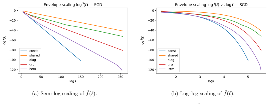
- [§6, Eq. (45) and Fig. 2] The empirical learnability window bH_N is constructed by applying the theoretical threshold ε_th^{emp}(ℓ;N), so Fig. 2 is not an independent corroboration of the detectability condition; it is a direct consequence of the definition. The scaling regimes are inferred from the envelope fits, and the predicted H_N then follows automatically. To validate the theory, the experiments should test a consequence that is not built in, for example by comparing bH_N against task-based recovery at each lag, by fitting the predicted exponents N(ℓ)∝f(ℓ)^{-κ_α}, or by varying N and measuring whether the lag at which task performance degrades matches the theoretical threshold. As written, the empirical section confirms internal consistency, not the central claim.
minor comments (6)
- [§5.4, Eq. (43)] The “master proportionality” N(ℓ)∝f(ℓ)^{-κ_α} is a rearrangement of Eq. (40) under the assumed model; calling it a proportionality relation is fine, but the paper should not present it as an additional derived law.
- [§5.1 and Eq. (28)] Earlier in the paper μ^{(q)}_{t,ℓ} may be signed (Eq. 14), but Eq. (28) and the surrounding text state μ^{(q)}_{t,ℓ}≥0. Please clarify whether the effective learning rates are always nonnegative after the diagonal projection or whether absolute values are intended.
- [Definition 5.1, Eq. (39)] If f(1)<ε_th(1), the set in (39) is empty. Please define H_N=0 in that case, consistent with the later statement “H_N may vanish identically”.
- [Appendix D, Eq. (58)–(62)] The LAN expansion is written for a single observation Y_N=θ+s_N Z, which is nonstandard. Please spell out the triangular-array formulation and state explicitly how the Fisher information I_α and the constant c_α are obtained for α-stable densities, since the main text says only “c_α>0 depends only on α”.
- [§6.1, Eq. (44)] The task lags are {32,64,128,192,256}, and the diagnostic grid is ℓ∈[4,256] with 128 uniform values. The boundary at ℓ=256 may truncate bH_N for GRU/LSTM; please report whether the observed saturation at ≈256 is an artifact of the grid limit.
- [General] Some references in the related-work discussion are cited for broad claims without page/theorem pointers (e.g., [21,30,38] for LAN of α-stable families). Adding precise statements or theorem numbers would help the reader verify the technical prerequisites.
Circularity Check
The empirical 'prediction' is constructed from the same theoretical threshold it is said to corroborate, and the master scaling law restates the assumed location model Δ∝f.
specific steps
-
self definitional
[Sec. 5.2–5.4, Eqs. (31), (33), (38), (39), (43)]
"Taking expectations over the randomness of the data yields E[S t,ℓ ] = P H q=1 µ(q) t,ℓ |mq(ℓ)| = mµ(ℓ)f(ℓ), (31) ... bSN (ℓ) | B ∼ SαS(θout, σα(ℓ)/N1−1/α), θout ∈ {+1/2 ∆(ℓ), −1/2 ∆(ℓ)} ,(33) ... the mean separation ∆(ℓ) = mµ(ℓ)f(ℓ) ... For a dependency at lag ℓ to be statistically detectable ... the envelope f(ℓ) must exceed εth(ℓ). ... The learnability window is H N = sup { ℓ≥1 : f(ℓ) ≥ εth(ℓ) } . (39)"
The location model is set up with the signal shift Δ=m_μ f, so f enters as the assumed mean amplitude; the threshold (38) is obtained by inverting the Fano bound for that shift; and H_N is then defined as the level set f≥ε_th. Consequently the master proportionality N∝f^{-κ}, the scaling laws, and the claim that slower envelope decay enlarges H_N are algebraic consequences of the definitions. The envelope is inserted as the signal and then recovered as the control variable, so the central qualitative prediction is built into the model's parameterization.
-
fitted input called prediction
[Sec. 6.1 Eq. (45); Sec. 6.2 results]
"we define the empirical learnability window as bH N = max { ℓ: fhat(ℓ) ≥ ε emp th (ℓ;N) } ,(45) where ε emp th (ℓ;N) denotes the empirical detectability threshold obtained by substituting αhat and σhatα(ℓ) into the theoretical criterion. This construction mirrors the definition of the theoretical learnability horizon H N. ... These behaviors are precisely those implied by the master proportionality N(ℓ) ∝ f(ℓ)^{-κα}, which links envelope geometry to sample complexity under heavy-tailed noise."
The empirical window bH_N is not an independently measured quantity; it is computed by applying the paper's own theoretical threshold (38) to the measured envelope with estimated α and σ. The observed saturation for exponentially decaying envelopes and expansion for slow envelopes is therefore forced by the construction: the output was defined through the same detectability relation that the experiments are said to corroborate. This is a fitted input being presented as a validated prediction.
full rationale
The formal part of the paper is a conditional mathematical derivation: if one accepts the SαS location model with mean shift Δ=m_μ f, then the Fano bound, the threshold, the window definition, and the scaling laws follow consistently. That part is not circular in itself, though the factorization in Eq. (31) treats the effective learning rates μ^{(q)}_{t,ℓ} as fixed coefficients when taking expectations, even though they are functions of the same input-dependent trajectory as the alignment variables ζ; as written, the key proportionality Δ∝f is partly assumed, not derived. The more clearly circular step is the empirical validation: Eq. (45) constructs bH_N by applying the theoretical threshold (38) to fitted envelope and noise quantities, and Sec. 6.2 then reports that the resulting curves 'confirm' the master proportionality. Because bH_N is defined by that same threshold, the empirical agreement is guaranteed up to the accuracy of the envelope/noise fits. The self-citations to [33] are used for the Jacobian product expansion and the multi-rate optimizer interpretation, but the expansion is restated in Appendix A using standard Fréchet calculus, so I do not treat those citations as load-bearing circularity. Overall score 6: the central empirical corroboration reduces by construction, and part of the theoretical signal-envelope relation is definitional, while the Fano/LAN analysis itself retains independent conditional content.
Axiom & Free-Parameter Ledger
free parameters (5)
- Envelope decay rate λ (exponential fits) =
ConstGate 0.68, SharedGate 0.39, DiagGate 0.020, GRU 0.018, LSTM 0.011
- Power-law exponent β (algebraic fits) =
DiagGate 1.71, GRU 1.59, LSTM 1.01
- Tail index α(ℓ) =
Architecture-dependent; near 2 for ConstGate/SharedGate, below 2 for DiagGate/GRU/LSTM
- Noise scale σ_α(ℓ) =
Lag-dependent, estimated per architecture
- Per-neuron time scales τ_q =
Fitted exponential decay constants per unit
axioms (9)
- domain assumption Gradient noise in deep learning is well modeled by symmetric α-stable laws with 1 ≤ α ≤ 2
- domain assumption The averaged matched statistic bS_N(ℓ) is in the domain of attraction of a symmetric α-stable law with scale σ_α(ℓ)/N^{1-1/α} and location ±Δ(ℓ)/2
- standard math LAN holds for shrinking-scale α-stable location families, yielding a KL lower bound with constant c_α
- standard math Fano's inequality and the KL–mutual-information mixture relation
- domain assumption Gate activations lie in [0,1] and activation derivatives are bounded in [0,1]
- domain assumption Alignment m_μ(ℓ) and noise scale σ_α(ℓ) are bounded above and below by positive constants over lags of interest
- domain assumption First-order expansion of Jacobian products (Eq. 12) is accurate and off-diagonal cross-neuron terms can be discarded
- domain assumption The fixed random projection w yields an unbiased probe of gradient geometry
- domain assumption Detectability of the matched statistic is necessary for learning a lag-ℓ dependency
invented entities (2)
-
Effective learning rate envelope f(ℓ)
independent evidence
-
Learnability window H_N
no independent evidence
read the original abstract
We develop a statistical theory of temporal learnability in recurrent neural networks, quantifying the maximal temporal horizon $\mathcal{H}_N$ over which gradient-based learning can recover lag-dependent structure at finite sample size $N$. The theory is built on the effective learning rate envelope $f(\ell)$, a function that captures how gating mechanisms and adaptive optimizers jointly shape the coupling between state-space dynamics and parameter updates during Backpropagation Through Time. Under heavy-tailed ($\alpha$-stable) fluctuations, where empirical averages concentrate at rate $N^{-1/\kappa_\alpha}$ with $\kappa_\alpha = \alpha/(\alpha-1)$, the interplay between envelope decay and statistical concentration yields explicit scaling laws for the growth of $\mathcal{H}_N$: logarithmic, polynomial, and exponential temporal learning regimes emerge according to the decay law of $f(\ell)$. These results identify envelope decay as the key determinant of temporal learnability. Slower attenuation of $f(\ell)$ enlarges $\mathcal{H}_N$, while heavy-tailed fluctuations compress it by weakening statistical concentration. Moreover, envelope geometry outweighs dataset size: slowing the envelope's decay enlarges $\mathcal{H}_N$ more than adding data, so more complex architectures that realize slower-decaying envelopes can be more data-efficient than simpler ones. Experiments across multiple gated architectures and optimizers corroborate these structural predictions.
Figures




Forward citations
Cited by 2 Pith papers
-
Anti-Collapse Dynamics and the Emergence of Multi-Time-Scale Learning in Recurrent Neural Networks
RNNs can sustain power-law forgetting and multi-time-scale learning when heavy-tailed fluctuations in SGD balance the collapse tendency toward short time scales, governed by a spectral exponent β.
-
Anti-Collapse Dynamics and the Emergence of Multi-Time-Scale Learning in Recurrent Neural Networks
A coarse-grained Levy-jump model predicts that recurrent networks settle into either a collapsed (exponential-forgetting) or anti-collapsed (power-law-forgetting) regime, with one spectral exponent beta governing both...
Reference graph
Works this paper leans on
-
[1]
Arjovsky, A
M. Arjovsky, A. Shah, and Y. Bengio. Unitary evolution recurrent neural networks. InInternational Conference on Machine Learning, pages 1120–1128, New York, USA, June 2016
2016
-
[2]
D. G. Barrett and B. Dherin. Implicit gradient regularization. InInternational Conference on Learning Representations, 2021
2021
-
[3]
Y. Bengio, P. Simard, and P. Frasconi. Learning long-term dependencies with gradient descent is difficult.IEEE Transactions on Neural Networks, 5(2):157–166, 1994. doi: 10.1109/72.279181
-
[4]
Antisymmetricrnn: Adynamical system view on recurrent neural networks
B.Chang, L.Meng, E.Haber, L.Ruthotto, D.Begert, andE.Holtham. Antisymmetricrnn: Adynamical system view on recurrent neural networks. InInternational Conference on Learning Representations, 2019
2019
-
[5]
Chang, Y
S. Chang, Y. Zhang, W. Han, M. Yu, X. Guo, W. Tan, X. Cui, M. Witbrock, M. Hasegawa-Johnson, and T. S. Huang. Dilated recurrent neural networks. InAdvances in Neural Information Processing Systems, 2017
2017
-
[6]
M. Chen, J. Pennington, and S. S. Schoenholz. Dynamical isometry and a mean field theory of RNNs: Gating enables signal propagation in recurrent neural networks. InProceedings of the 35th International Conference on Machine Learning, pages 872–881, 2018
2018
-
[7]
Chezhegov, K
S. Chezhegov, K. Yaroslav, A. Semenov, A. Beznosikov, A. Gasnikov, S. Horváth, M. Takáč, and E. Gorbunov. Clipping improves Adam-norm and AdaGrad-norm when the noise is heavy-tailed. In A. Singh, M. Fazel, D. Hsu, S. Lacoste-Julien, F. Berkenkamp, T. Maharaj, K. Wagstaff, and J. Zhu, editors,Proceedings of the 42nd International Conference on Machine Lear...
2025
-
[8]
K. Cho, B. Van Merriënboer, D. Bahdanau, and Y. Bengio. On the properties of neural machine translation: Encoder-decoder approaches.arXiv preprint arXiv:1409.1259, 2014
Pith/arXiv arXiv 2014
-
[9]
Chung, S
J. Chung, S. Ahn, and Y. Bengio. Hierarchical multiscale recurrent neural networks. InInternational Conference on Learning Representations, Toulon, France, Apr. 2017
2017
-
[10]
Cooijmans, N
T. Cooijmans, N. Ballas, C. Laurent, C. Gülçehre, and A. C. Courville. Recurrent batch normalization. InInternational Conference on Learning Representations, 2016
2016
-
[11]
T. M. Cover and J. A. Thomas.Elements of Information Theory. John Wiley & Sons, New York, NY,
-
[12]
J. Dambre, D. Verstraeten, B. Schrauwen, and S. Massar. Information processing capacity of dynamical systems.Scientific Reports, 2, 2012. doi: 10.1038/srep00514
-
[13]
T. Dao, G. Yang, S. L. Smith, and L. Amini. Kernel regime of wide neural networks: Gradient descent dynamics and generalization. InAdvances in Neural Information Processing Systems, 2021
2021
-
[14]
F. A. Gers, J. Schmidhuber, and F. Cummins. Learning to forget: Continual prediction with LSTM. InNeural Computation, volume 12, pages 2451–2471, 2000
2000
-
[15]
A. Gu, I. Johnson, K. Goel, K. K. Saab, T. Dao, A. Rudra, and C. Ré. Combining recurrent, convolu- tional, and continuous-time models with linear state space layers. InThirty-Fifth Conference on Neural Information Processing Systems, 2021
2021
-
[16]
A. Gu, K. Goel, and C. Ré. Efficiently modeling long sequences with structured state spaces. In International Conference on Learning Representations, 2022. 38
2022
-
[17]
Gupta, H
H. Gupta, H. Mehta, and J. Z. Kolter. Stability and expressivity of implicit recurrent models. In Advances in Neural Information Processing Systems, 2022
2022
-
[18]
N. J. Higham.Functions of Matrices: Theory and Computation. SIAM, 2008
2008
-
[19]
Hochreiter and J
S. Hochreiter and J. Schmidhuber. Long short-term memory.Neural Computation, 9(8):1735–1780, 1997
1997
-
[20]
Hübler, I
F. Hübler, I. Fatkhullin, and N. He. From gradient clipping to normalization for heavy tailed SGD,
-
[21]
I. A. Ibragimov and R. Z. Has’minskii.Statistical Estimation: Asymptotic Theory. Springer, New York, 1981
1981
-
[22]
H. Jaeger. Short term memory in echo state networks. Technical Report GMD Report 152, Fraunhofer Institute for Autonomous Intelligent Systems, 2002
2002
-
[23]
Jastrzebski, Z
S. Jastrzebski, Z. Kenton, D. Arpit, N. Ballas, V. Verma, K. Cheung, and Y. Bengio. Three factors influencing minima in SGD. InICLR Workshop, 2017
2017
-
[24]
L. Jing, D. C. Gürsoy, T. Laurent, Y. LeCun, and Y. Bengio. Tunable efficient unitary neural networks (eunn) and their application to rnns. InInternational Conference on Machine Learning, 2017
2017
-
[25]
D. P. Kingma and J. Ba. Adam: A method for stochastic optimization, 2017. URLhttps://arxiv. org/abs/1412.6980
Pith/arXiv arXiv 2017
-
[26]
Koutnik, K
J. Koutnik, K. Greff, F. Gomez, and J. Schmidhuber. A clockwork RNN. InInternational Conference on Machine Learning, volume 32, pages 1863–1871, 2014
2014
-
[27]
S. G. Krantz and H. R. Parks.The Implicit Function Theorem: History, Theory, and Applications. Birkhäuser, Boston, MA, 2003. doi: 10.1007/978-0-8176-8230-9
-
[28]
K. Krishnamurthy, T. Can, and D. J. Schwab. Theory of gating in recurrent neural networks.Physical Review X, 12(1):011011, 2022. doi: 10.1103/PhysRevX.12.011011
-
[29]
Q. V. Le, N. Jaitly, and G. E. Hinton. A simple way to initialize recurrent networks of rectified linear units. InarXiv preprint arXiv:1504.00941, 2015
Pith/arXiv arXiv 2015
-
[30]
Le Cam and G
L. Le Cam and G. L. Yang.Asymptotics in Statistics: Some Basic Concepts. Springer, New York, 2000
2000
-
[31]
H. Li, Z. Xu, G. Taylor, C. Studer, and T. Goldstein. Visualizing the loss landscape of neural nets. Advances in Neural Information Processing Systems, 2018
2018
-
[32]
Z. Liu. Online convex optimization with heavy tails: Old algorithms, new regrets, and applications,
-
[33]
L. Livi. Time-scale coupling between states and parameters in recurrent neural networks.arXiv preprint arXiv:2508.12121, 2025. doi: 10.48550/arXiv.2508.12121. URLhttps://arxiv.org/abs/2508.12121
-
[34]
URLhttps://arxiv.org/abs/2508.07473
-
[35]
J. Martens. New insights and perspectives on the natural gradient method.arXiv preprint arXiv:1412.1193, 2014
Pith/arXiv arXiv 2014
-
[36]
Loshchilov and F
I. Loshchilov and F. Hutter. Decoupled weight decay regularization.International Conference on Learning Representations, 2019
2019
-
[37]
J. H. McCulloch. Simple consistent estimators of stable distribution parameters.Communications in Statistics–Simulation and Computation, 15(4):1109–1136, 1986
1986
-
[38]
S. McCandlish, J. Kaplan, and D. Amodei. An empirical model of large-batch training.arXiv preprint arXiv:1812.06162, 2018. 39
Pith/arXiv arXiv 2018
-
[39]
Pascanu, T
R. Pascanu, T. Mikolov, and Y. Bengio. On the difficulty of training recurrent neural networks. In Proceedings of the 30th International Conference on Machine Learning, volume 28, pages 1310–1318, Atlanta, Georgia, USA, 2013
2013
-
[40]
J. P. Nolan.Univariate Stable Distributions: Models for Heavy Tailed Data. Springer Series in Opera- tions Research and Financial Engineering. Springer, Cham, 2020. ISBN 978-3-030-52917-8. Print ISBN: 978-3-030-52917-8; eBook ISBN: 978-3-030-52918-5
2020
-
[41]
Rubanova, R
Y. Rubanova, R. T. Chen, and D. Duvenaud. Latent ordinary differential equations for irregularly- sampled time series. InAdvances in Neural Information Processing Systems, 2019
2019
-
[42]
Pennington, S
J. Pennington, S. Schoenholz, and S. Ganguli. Resurrecting the sigmoid in deep learning through dynamical isometry: theory and practice. InAdvances in Neural Information Processing Systems, pages 4785–4795, 2017
2017
-
[43]
A. M. Saxe, J. L. McClelland, and S. Ganguli. Exact solutions to the nonlinear dynamics of learning in deep linear neural networks.arXiv preprint arXiv:1312.6120, 2013
Pith/arXiv arXiv 2013
-
[44]
S. Ruder. An overview of gradient descent optimization algorithms.arXiv preprint arXiv:1609.04747, 2016
Pith/arXiv arXiv 2016
-
[45]
Simsekli, L
U. Simsekli, L. Sagun, and M. Gurbuzbalaban. A tail-index analysis of stochastic gradient noise in deep neural networks. InAdvances in Neural Information Processing Systems, pages 1–12, 2019
2019
-
[46]
R. Shwartz-Ziv and N. Tishby. Opening the black box of deep neural networks via information.arXiv preprint arXiv:1703.00810, 2017
Pith/arXiv arXiv 2017
-
[47]
Tallec and Y
C. Tallec and Y. Ollivier. Can recurrent neural networks warp time? InInternational Conference on Learning Representations, 2018
2018
-
[48]
S. L. Smith and Q. V. Le. A bayesian perspective on generalization and stochastic gradient descent. In International Conference on Learning Representations, 2018
2018
-
[49]
P. Verzelli, C. Alippi, and L. Livi. Echo state networks with self-normalizing activations on the hyper- sphere.Scientific Reports, 9:13887, 2019. doi: 10.1038/s41598-019-50158-4
-
[50]
A. W. van der Vaart.Asymptotic Statistics. Cambridge University Press, 1998
1998
-
[51]
Yang and E
G. Yang and E. Hu. Tensor programs v: Tuning large neural networks via zero-shot hyperparameter transfer. InAdvances in Neural Information Processing Systems, 2021
2021
-
[52]
Wisdom, T
S. Wisdom, T. Powers, J. R. Hershey, J. Le Roux, and L. E. Atlas. Full-capacity unitary recurrent neural networks. InAdvances in Neural Information Processing Systems, 2016
2016
-
[53]
Zhang, A
J. Zhang, A. M. Saxe, M. S. Advani, and A. Lee. Improving the trainability of deep networks by standardizing the gradient. InInternational Conference on Machine Learning, 2020
2020
-
[54]
Zhang, S
C. Zhang, S. Bengio, and Y. Singer. Are all layers created equal?Journal of Machine Learning Research, 23(67):1–28, 2022
2022
-
[56]
P. Zhou, J. Feng, C. Ma, C. Xiong, S. C. H. Hoi, and W. E. Towards theoretically understanding why SGD generalizes better than adam in deep learning. In H. Larochelle, M. Ranzato, R. Hadsell, M. Balcan, and H. Lin, editors,Advances in Neural Information Processing Systems, volume 33, pages 21285–21296. Curran Associates, Inc., 2020. 40
2020
-
[2025]
URLhttps://arxiv.org/abs/2410.13849
discussion (0)
Sign in with ORCID, Apple, or X to comment. Anyone can read and Pith papers without signing in.