REVIEW 4 major objections 4 minor 1 cited by
The paper claims that optimal control of obstacle problems can be solved mesh-free by constraint-embedding neural networks, trained with a single-loop stochastic algorithm whose Moreau-penalized objective converges at O(K^{-(1-p)/2}).
Reviewed by Pith at T0; open to challenge. T0 means a machine referee read the full paper against a public rubric. the ladder, T0–T4 →
T0 review · deepseek-v4-flash
2026-08-03 12:06 UTC pith:B54VWAM6
load-bearing objection A useful single-loop algorithm for bilevel obstacle control, but the convergence theorem only reaches a penalized stationarity point, not the true bilevel solution, and the paper leaves that gap open. the 4 major comments →
A Single-Loop Bilevel Deep Learning Method for Optimal Control of Obstacle Problems
The pith
A machine-rendered reading of the paper's core claim, the machinery that carries it, and where it could break.
Core claim
The paper's central claim is that the bilevel optimal control problem (2.1) can be approximated by a stochastic bilevel problem over neural-network parameters (3.5), and that S2-FOBA solves that problem without nested optimization. The Moreau-envelope reformulation replaces the lower-level constraint with e(θ_y, θ_u) ≤ e_γ(θ_y, θ_u), where e_γ is a continuously differentiable Moreau envelope whose proximal center is tracked by an auxiliary variable z_k. The algorithm minimizes the penalized objective φ_c(θ) = j(θ)/c + (e(θ) − e_γ(θ)) by alternating stochastic gradient steps for z, θ_y, and θ_u in one loop. Theorem 4.1 states that under ρ-weak convexity and Lipschitz smoothness, with step siz
What carries the argument
The central mechanism is the Moreau-envelope-based reformulation: the bilevel constraint θ_y ∈ arg min e(θ_y, θ_u) is replaced by e(θ_y, θ_u) ≤ e_γ(θ_y, θ_u), where e_γ is the Moreau envelope e_γ(θ_y, θ_u) = min_z {e(z, θ_u) + (1/2γ)||z − θ_y||^2}. This converts the constraint into a smooth penalty ψ_c = j + c(e − e_γ), avoiding the nonsmooth value function. The constraint-embedding network architectures (3.1)–(3.4) bake the obstacle and control constraints directly into the network output, so no penalty or active-set detection is needed for feasibility. The auxiliary sequence z_k approximates the proximal center z*_γ and is updated inside the same loop, which eliminates the inner minimizati
Load-bearing premise
The argument depends on the assumption that a point where the lower-level network's objective has zero gradient is actually a global minimizer of that objective; the paper establishes this when the lower level is convex in the state parameters, but the implemented neural network is explicitly nonconvex.
What would settle it
Construct a small lower-level network whose energy has two well-separated local minima for a fixed control parameter (e.g., a one-dimensional parameter with two energy wells), run S2-FOBA with the stated step sizes, and test whether the returned state parameter satisfies the lower-level optimality condition min_z e(z, θ_u) approximately. If the gradient of the penalized objective is small while e(θ_y, θ_u) stays above the true minimum, the convergence measure has decoupled from feasibility.
If this is right
- With trained networks, evaluating the solution at a new mesh is only a forward pass, whereas classical active-set methods require re-meshing and re-solving; the paper's Table 5.2 shows order-of-magnitude time savings at moderate resolutions.
- The bilevel training avoids the failure mode of weighted single-level objectives such as (2.4), which cannot produce a state that minimizes the lower-level energy for the computed control.
- The two-stage refinement restores lower-level feasibility of the state for the Stage-1 control, yielding relative L2 errors around 1e-2 to 1e-3 in the benchmarks.
- Because S2-FOBA needs only first-order stochastic gradients and does not assume lower-level uniqueness, it implements as a single loop and scales to larger networks and domains than nested-solve approaches.
- The same algorithm extends to obstacle control and to optimal control of elliptic variational inequalities by replacing the lower-level loss with a projection fixed-point residual.
Where Pith is reading between the lines
- Inference: Theorem 4.1 bounds the gradient of the penalized Moreau objective, not the gap to the original bilevel optimum. If the lower-level network has spurious stationary points, the stated rate could hold while the control remains suboptimal; the practical value then depends on how often Stage 2's refinement is needed.
- Inference: Stage 2 repairs only the state, never the control. If Stage 1 returns a poor control, the refinement cannot fix it, so end-to-end accuracy relies on Stage 1 having already found a good control.
- Inference: The mesh-free nature suggests a natural extension to three-dimensional or higher-dimensional domains, where classical active-set methods would become expensive and where the paper's complex-domain experiments hint that the method's error would remain roughly mesh-independent.
- Inference: The manual choices of step sizes and penalty schedules (e.g., c_k = 5k^0.3) leave room for automated tuning; testing a wider range of growth exponents would separate the method's robustness from its sensitivity to these hyperparameters.
Editorial analysis
A structured set of objections, weighed in public.
Referee Report
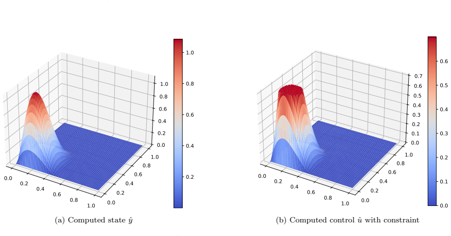
Summary. The paper proposes a mesh-free bilevel deep learning method for optimal control of obstacle problems. The state and control are parameterized by constraint-embedding neural networks, and the resulting stochastic bilevel problem (3.5) is solved by a single-loop stochastic first-order algorithm (S2-FOBA) based on the Moreau-envelope reformulation (3.6) and a penalty strategy (3.10). The main theoretical result, Theorem 4.1, states that S2-FOBA drives the gradient of the penalized objective φ_{c_k} to zero at rate O(1/K^{(1-p)/2}) under assumptions A1–A3. Numerical experiments on benchmark obstacle-control problems, including control-constrained, irregular-domain, obstacle-control, and EVI examples, report relative L2 errors in the range 4e-3 to 3e-2 and favorable cost comparisons against an active-set method. A two-stage refinement (Algorithm 3.2) is added to improve lower-level feasibility of the final state.
Significance. If the convergence claim is interpreted as convergence to stationarity of the Moreau-penalized surrogate, the paper offers a useful single-loop, Hessian-free, stochastic algorithm for a hard nonsmooth bilevel problem class. The method is mesh-free, handles complex domains, and is supported by reproducible PyTorch code and comparisons with classical active-set and MPEC solvers. The authors also correctly identify and demonstrate the failure of naive objective-combination approaches. However, the paper's stronger claim that S2-FOBA solves the original obstacle-control problem (2.1) is not justified by the analysis as written: Theorem 4.1 controls only the gradient of φ_{c_k}, and the connection between φ_{c_k} and the original bilevel problem relies on an equivalence that the paper itself states requires lower-level convexity, which is not satisfied by the implemented nonconvex neural-network parametrization.
major comments (4)
- [§3.2.1 and Theorem 4.1] The load-bearing equivalence between (3.6) and (3.5) is stated by the authors to hold only when the stationary set of e(·, θu) coincides with its minimizer set, 'which holds, for instance, when e is convex in θy'. But §3.1 states that the lower-level problem is 'in general, nonconvex'. For nonconvex e, equality in the Moreau constraint e ≤ e_γ is equivalent to lower-level stationarity, not global minimality. Theorem 4.1 bounds E‖∇φ_{c_k}‖ and does not control the feasibility gap e − e_γ. Thus the paper does not establish that S2-FOBA produces a feasible lower-level minimizer for the original problem, even in the deterministic zero-variance limit. This gap should be addressed either by restricting the theoretical result to the stationarity-based surrogate, or by adding a mechanism that guarantees convergence to a true lower-level minimizer.
- [Assumptions A1–A2 and §3.1] Theorem 4.1 assumes ρ-weak convexity and L_e-smoothness of the NN lower-level objective e(θy,θu) in (3.5). For the implemented ResNet with Swish activations and the constraint-embedding maps (3.1)–(3.3), these properties are not verified. In particular, global weak convexity in θy is not generally inherited by deep residual networks. The paper should either prove or state sufficient architecture conditions under which A1–A2 hold, or explicitly frame the convergence analysis as conditional on these assumptions and discuss their plausibility for the tested networks.
- [§3.3, Stage 2] Stage 2 of Algorithm 3.2 re-solves the lower-level problem only for the final control parameter θ̃u, using θ̂y as initialization. This can only repair the state; it cannot repair a control that Stage 1 selected while the state parameter was at a spurious stationary point of the nonconvex lower-level objective. Consequently, the two-stage procedure does not restore feasibility of the coupled bilevel pair. The numerical examples may still be meaningful, but the paper should clarify that the method is not guaranteed to enforce bilevel feasibility, and should report any empirical check of lower-level optimality (e.g., comparison of e(θ̂y,θ̃u) with the value obtained by a full lower-level solve).
- [§5, Tables 5.1–5.2] The numerical results are reported for a fixed network architecture and fixed hyperparameters (γ, c_k, learning rates), and the convergence theorem's step-size conditions are not checked in the experiments. Since the theory is a central advertised contribution, the paper should at least discuss how the selected step-size and penalty schedules relate to the assumptions of Theorem 4.1, or state that the experiments are heuristic. This does not invalidate the numerical evidence, but it weakens the connection between theory and practice.
minor comments (4)
- [§5, Figure 5.4 caption] Typo: 'Comparions' should be 'Comparisons'.
- [§6.3, text near Eq. (6.5)] Missing space in 'lossein'; also 'we set η=0.01' redefines the symbol η already used for step sizes, which can be confusing.
- [§2.1] The notation 'Gˆ ateaux' in the introduction has a corrupted accent; should be 'Gâteaux'.
- [§4.1, Assumption A1] The symbols θ := (θy, θu) are introduced after Assumption A1, but A1 already uses θy,θu jointly; the ordering of definitions could be improved.
Circularity Check
No circular reduction: Theorem 4.1 is a genuine stationarity-convergence result, and the numerical claims are benchmarked against independent solvers; the self-cited Moreau-envelope lemmas are independent mathematical support, not fitted inputs.
full rationale
The derivation chain is not circular. The central theorem, Theorem 4.1, is proved in Section 4 via explicit descent inequalities for the merit function φ_c; it concludes convergence to a stationary point of the penalized Moreau objective, and that conclusion is not obtained by fitting a parameter to the target outputs. The numerical results are validated against independent classical solvers and analytical solutions (active-set method [26], MPEC reference [28]), so the reported errors are not constructed from the training data. The Moreau-envelope machinery is imported from the authors' own prior work, [21] and [39], and this is the main self-citation burden; however, the cited results are parameter-free lemmas/theorems with stated assumptions (ρ-weak convexity, γ < 1/ρ, etc.) and do not already contain the paper's target result, so they qualify as independent support under the review rules. A real limitation, acknowledged by the paper itself, is that the reformulation (3.6) is equivalent to (3.5) only when the lower-level stationary set coincides with the minimizer set: Section 3.2.1 states this equivalence "holds, for instance, when e is convex with respect to θy", while Section 3.1 notes "the lower-level problem is, in general, nonconvex". This creates a semantic gap between convergence to a stationary point of φ_c and actually solving the bilevel problem (2.1), but it is a correctness/feasibility limitation, not a circularity, because Theorem 4.1 does not claim equivalence to (2.1) and the convergence result is not defined in terms of the original problem's solution.
Axiom & Free-Parameter Ledger
free parameters (5)
- proximal parameter γ =
20 (Ex.1), 500 (Ex.2), 50 (Ex.3, Ex.4), 200000 (Ex.5)
- penalty parameter sequence c_k =
5k^0.3 (Ex.1,2,5), 5k^0.2 (Ex.3), (1/5)k^0.2 (Ex.4)
- learning rates α, β, η =
1e-3 with 0.8 decay per 1000 epochs (Ex.1-4); 2e-4 (Ex.5)
- mini-batch size m =
512 for most examples
- NN architecture (depth/width/activation) =
ResNet, 3 residual blocks, 16 neurons per layer, Swish
axioms (5)
- ad hoc to paper The NN lower-level objective e in (3.5) is ρ-weakly convex in (θy, θu) and L_e-smooth (A1-A2).
- ad hoc to paper Stationary points of the lower-level NN problem coincide with its minimizers, making (3.6) equivalent to (3.5).
- domain assumption Deep Ritz / universal approximation: minimizing the NN energy produces a state solving the obstacle problem, so the NN bilevel problem (3.5) approximates the continuous problem (2.1).
- domain assumption Stochastic gradient oracles are unbiased with bounded variance (A3).
- standard math Solution existence for (2.1) and standard Moreau-envelope properties from [39].
read the original abstract
Optimal control of obstacle problems arises in a wide range of applications and is computationally challenging due to its nonsmoothness, nonlinearity, and bilevel structure. Classical numerical approaches rely on mesh-based discretization and typically require solving a sequence of costly subproblems. In this work, we propose a single-loop bilevel deep learning method, which is mesh-free, scalable to high-dimensional and complex domains, and avoids repeated solution of discretized subproblems. The method employs constraint-embedding neural networks to approximate the state and control and preserves the bilevel structure. To train the neural networks efficiently, we propose a Single-Loop Stochastic First-Order Bilevel Algorithm (S2-FOBA), which eliminates nested optimization and does not rely on restrictive lower-level uniqueness assumptions. We analyze the convergence behavior of S2-FOBA under mild assumptions. Numerical experiments on benchmark examples, including distributed and obstacle control problems with regular and irregular obstacles on complex domains, demonstrate that the proposed method achieves satisfactory accuracy while reducing computational cost compared to classical numerical methods.
Figures




Forward citations
Cited by 1 Pith paper
-
Constrained Neural Parameterization for Optimization in Function Spaces
Neural parameterizations are constructed whose range lies in admissible sets for function-space optimization, converting constrained problems to unconstrained gradient-based ones.
Reference graph
Works this paper leans on
-
[1]
A. Alphonse, M. Hinterm \"u ller, A. Kister, C. H. Lun, and C. Sirotenko , A neural network approach to learning solutions of a class of elliptic variational inequalities , arXiv preprint arXiv:2411.18565, (2024)
Pith/arXiv arXiv 2024
-
[2]
Barbu , Optimal control of variational inequalities , Research Notes in Math., 100 (1984)
V. Barbu , Optimal control of variational inequalities , Research Notes in Math., 100 (1984)
1984
-
[3]
Barry-Straume, A
J. Barry-Straume, A. Sarshar, A. A. Popov, and A. Sandu , Physics-informed neural networks for PDE-constrained optimization and control , Communications on Applied Mathematics and Computation, (2025), pp. 1--24
2025
-
[4]
Bergounioux , Use of augmented Lagrangian methods for the optimal control of obstacle problems , Journal of Optimization Theory and Applications, 95 (1997), pp
M. Bergounioux , Use of augmented Lagrangian methods for the optimal control of obstacle problems , Journal of Optimization Theory and Applications, 95 (1997), pp. 101--126
1997
-
[5]
Bergounioux and S
M. Bergounioux and S. Lenhart , Optimal control of bilateral obstacle problems , SIAM Journal on Control and Optimization, 43 (2004), pp. 240--255
2004
-
[6]
Bourgat and G
J. Bourgat and G. Duvaut , Numerical analysis of flow with or without wake past a symmetric two-dimensional profile without incidence , International Journal for Numerical Methods in Engineering, 11 (1977), pp. 975--993
1977
-
[7]
u ller, and C. L \
C. Brett, C. M. Elliott, M. Hinterm \"u ller, and C. L \"o bhard , Mesh adaptivity in optimal control of elliptic variational inequalities with point-tracking of the state , Interfaces and Free Boundaries, 17 (2015), pp. 21--53
2015
-
[8]
Brezis and G
H. Brezis and G. Stampacchia , The hodograph method in fluid-dynamics in the light of variational inequalities , Archive for Rational Mechanics and Analysis, 61 (1976), pp. 1--18
1976
-
[9]
Y. Cao, C. C. So, Y. Dai, S. P. Yung, and J.-M. Wang , Adversarial physics-informed neural networks with hard constraints for optimal control of PDEs , Journal of Computational Physics, 541 (2025), p. 114307
2025
-
[10]
T. Chen, Y. Sun, and W. Yin , Closing the gap: Tighter analysis of alternating stochastic gradient methods for bilevel problems , Advances in Neural Information Processing Systems, 34 (2021), pp. 25294--25307
2021
-
[11]
Cheng, X
X. Cheng, X. Shen, X. Wang, and K. Liang , A deep neural network-based method for solving obstacle problems , Nonlinear Analysis: Real World Applications, 72 (2023), p. 103864
2023
-
[12]
P. L. Combettes and J.-C. Pesquet , Deep neural network structures solving variational inequalities , Set-Valued and Variational Analysis, 28 (2020), pp. 491--518
2020
-
[13]
C. W. Cryer , The method of Christopherson for solving free boundary problems for infinite journal bearings by means of finite differences , Mathematics of Computation, 25 (1971), pp. 435--443
1971
-
[14]
Cybenko , Approximation by superpositions of a sigmoidal function , Mathematics of Control, Signals and Systems, 2 (1989), pp
G. Cybenko , Approximation by superpositions of a sigmoidal function , Mathematics of Control, Signals and Systems, 2 (1989), pp. 303--314
1989
-
[15]
Darehmiraki , A deep learning approach for the obstacle problem , in Proceedings of Academia-Industry Consortium for Data Science: AICDS 2020, Springer, 2022, pp
M. Darehmiraki , A deep learning approach for the obstacle problem , in Proceedings of Academia-Industry Consortium for Data Science: AICDS 2020, Springer, 2022, pp. 179--188
2020
-
[16]
De Los Reyes , On the optimal control of some nonsmooth distributed parameter systems arising in mechanics , GAMM-Mitteilungen, 40 (2018), pp
J.-C. De Los Reyes , On the optimal control of some nonsmooth distributed parameter systems arising in mechanics , GAMM-Mitteilungen, 40 (2018), pp. 268--286
2018
-
[17]
W. E and B. Yu , The deep Ritz method: A deep learning-based numerical algorithm for solving variational problems , Communications in Mathematics and Statistics, 6 (2018), pp. 1--12
2018
-
[18]
El Bahja, J
H. El Bahja, J. C. Hauffen, P. Jung, B. Bah, and I. Karambal , A physics-informed neural network framework for modeling obstacle-related equations , Nonlinear Dynamics, 113 (2025), pp. 1--12
2025
-
[19]
Friedman , Variational Principles and Free-Boundary Problems , Dover Books on Mathematics, Dover Publications, 2010
A. Friedman , Variational Principles and Free-Boundary Problems , Dover Books on Mathematics, Dover Publications, 2010
2010
-
[20]
u ller, R. H. Hoppe, and C. L \
A. Gaevskaya, M. Hinterm \"u ller, R. H. Hoppe, and C. L \"o bhard , Adaptive finite elements for optimally controlled elliptic variational inequalities of obstacle type , in Optimization with PDE Constraints: ESF networking program'OPTPDE', Springer, 2014, pp. 95--150
2014
-
[21]
L. L. Gao, J. J. Ye, H. Yin, S. Zeng, and J. Zhang , Moreau envelope based difference-of-weakly-convex reformulation and algorithm for bilevel programs , arXiv preprint arXiv:2306.16761, (2023)
Pith/arXiv arXiv 2023
-
[22]
Y. Gao, Y. Song, Z. Tan, H. Yue, and S. Zeng , Prox-PINNs : A deep learning algorithmic framework for elliptic variational inequalities , arXiv preprint arXiv:2505.14430, (2025)
arXiv 2025
-
[23]
Glowinski , Lectures on Numerical Methods for Non-Linear Variational Problems , Springer Science & Business Media, 2008
R. Glowinski , Lectures on Numerical Methods for Non-Linear Variational Problems , Springer Science & Business Media, 2008
2008
-
[24]
Glowinski , Variational Methods for the Numerical Solution of Nonlinear Elliptic Problems , SIAM, 2015
R. Glowinski , Variational Methods for the Numerical Solution of Nonlinear Elliptic Problems , SIAM, 2015
2015
-
[25]
Z. Hao, C. Ying, H. Su, J. Zhu, J. Song, and Z. Cheng , Bi-level physics-informed neural networks for PDE constrained optimization using Broyden's hypergradients , The 11th International Conference on Learning Representations, (2023)
2023
-
[26]
M. Hinterm \"u ller , An active-set equality constrained Newton solver with feasibility restoration for inverse coefficient problems in elliptic variational inequalities , Inverse Problems, 24 (2008), p. 034017
2008
-
[27]
u ller, R. H. Hoppe, and C. L \
M. Hinterm \"u ller, R. H. Hoppe, and C. L \"o bhard , Dual-weighted goal-oriented adaptive finite elements for optimal control of elliptic variational inequalities , ESAIM: Control, Optimisation and Calculus of Variations, 20 (2014), pp. 524--546
2014
-
[28]
Hinterm \"u ller and I
M. Hinterm \"u ller and I. Kopacka , Mathematical programs with complementarity constraints in function space: C-and strong stationarity and a path-following algorithm , SIAM Journal on Optimization, 20 (2009), pp. 868--902
2009
-
[29]
Hinterm \"u ller and I
M. Hinterm \"u ller and I. Kopacka , A smooth penalty approach and a nonlinear multigrid algorithm for elliptic MPECs , Computational Optimization and Applications, 50 (2011), pp. 111--145
2011
-
[30]
u ller, C. L \
M. Hinterm \"u ller, C. L \"o bhard, and M. Tber , An ^1 -penalty scheme for the optimal control of elliptic variational inequalities , in Numerical Analysis and Optimization: NAO-III, Muscat, Oman, January 2014, Springer, 2015, pp. 151--190
2014
-
[31]
Hinterm \"u ller and T
M. Hinterm \"u ller and T. Surowiec , A bundle-free implicit programming approach for a class of elliptic MPECs in function space , Mathematical Programming, 160 (2016), pp. 271--305
2016
-
[32]
Hornik , Approximation capabilities of multilayer feedforward networks , Neural Networks, 4 (1991), pp
K. Hornik , Approximation capabilities of multilayer feedforward networks , Neural Networks, 4 (1991), pp. 251--257
1991
-
[33]
Hornik, M
K. Hornik, M. Stinchcombe, and H. White , Multilayer feedforward networks are universal approximators , Neural Networks, 2 (1989), pp. 359--366
1989
-
[34]
Ito and K
K. Ito and K. Kunisch , Semi-smooth Newton methods for variational inequalitiesof the first kind , ESAIM: Mathematical Modelling and Numerical Analysis, 37 (2003), pp. 41--62
2003
-
[35]
Ito and K
K. Ito and K. Kunisch , Optimal control of obstacle problems by H^1 -obstacles , Applied Mathematics and Optimization, 56 (2007), pp. 1--17
2007
-
[36]
Jaillet, D
P. Jaillet, D. Lamberton, and B. Lapeyre , Variational inequalities and the pricing of American options , Acta Applicandae Mathematica, 21 (1990), pp. 263--289
1990
-
[37]
Kinderlehrer and G
D. Kinderlehrer and G. Stampacchia , An Introduction to Variational Inequalities and Their Applications , SIAM, 2000
2000
-
[38]
M.-C. Lai, Y. Song, X. Yuan, H. Yue, and T. Zeng , The hard-constraint PINNs for interface optimal control problems , SIAM Journal on Scientific Computing, 47 (2025), pp. C601--C629
2025
-
[39]
R. Liu, Z. Liu, W. Yao, S. Zeng, and J. Zhang , Moreau envelope for nonconvex bi-level optimization: A single-loop and Hessian -free solution strategy , in International Conference on Machine Learning, PMLR, 2024, pp. 31566--31596
2024
-
[40]
L. Lu, R. Pestourie, W. Yao, Z. Wang, F. Verdugo, and S. G. Johnson , Physics-informed neural networks with hard constraints for inverse design , SIAM Journal on Scientific Computing, 43 (2021), pp. B1105--B1132
2021
-
[41]
D. Luo, T. O’Leary-Roseberry, P. Chen, and O. Ghattas , Efficient PDE-constrained optimization under high-dimensional uncertainty using derivative-informed neural operators , SIAM Journal on Scientific Computing, 47 (2025), pp. C899--C931
2025
-
[42]
Meyer, A
C. Meyer, A. Rademacher, and W. Wollner , Adaptive optimal control of the obstacle problem , SIAM Journal on Scientific Computing, 37 (2015), pp. A918--A945
2015
-
[43]
Meyer and O
C. Meyer and O. Thoma , A priori finite element error analysis for optimal control of the obstacle problem , SIAM Journal on Numerical Analysis, 51 (2013), pp. 605--628
2013
-
[44]
Mignot , Contr \^o le dans les in \'e quations variationelles elliptiques , Journal of Functional Analysis, 22 (1976), pp
F. Mignot , Contr \^o le dans les in \'e quations variationelles elliptiques , Journal of Functional Analysis, 22 (1976), pp. 130--185
1976
-
[45]
Mignot and J
F. Mignot and J. P. Puel , Optimal control in some variational inequalities , SIAM Journal on Control and Optimization, 22 (1984), pp. 466--476
1984
-
[46]
Mowlavi and S
S. Mowlavi and S. Nabi , Optimal control of PDEs using physics-informed neural networks , Journal of Computational Physics, 473 (2023), p. 111731
2023
-
[47]
Nemirovski, A
A. Nemirovski, A. Juditsky, G. Lan, and A. Shapiro , Robust stochastic approximation approach to stochastic programming , SIAM Journal on Optimization, 19 (2009), pp. 1574--1609
2009
-
[48]
Raissi, P
M. Raissi, P. Perdikaris, and G. E. Karniadakis , Physics-informed neural networks: A deep learning framework for solving forward and inverse problems involving nonlinear partial differential equations , Journal of Computational Physics, 378 (2019), pp. 686--707
2019
-
[49]
Schiela and D
A. Schiela and D. Wachsmuth , Convergence analysis of smoothing methods for optimal control of stationary variational inequalities with control constraints , ESAIM: Mathematical Modelling and Numerical Analysis, 47 (2013), pp. 771--787
2013
-
[50]
Sirignano and K
J. Sirignano and K. Spiliopoulos , DGM : A deep learning algorithm for solving partial differential equations , Journal of Computational Physics, 375 (2018), pp. 1339--1364
2018
-
[51]
Y. Song, X. Yuan, and H. Yue , Accelerated primal-dual methods with enlarged step sizes and operator learning for nonsmooth optimal control problems , arXiv preprint arXiv:2307.00296, (2023)
Pith/arXiv arXiv 2023
-
[52]
Y. Song, X. Yuan, and H. Yue , The ADMM-PINNs algorithmic framework for nonsmooth PDE-constrained optimization: A deep learning approach , SIAM Journal on Scientific Computing, 46 (2024), pp. C659--C687
2024
-
[53]
Y. Song, X. Yuan, H. Yue, and T. Zeng , An operator learning approach to nonsmooth optimal control of nonlinear PDEs , arXiv preprint arXiv:2409.14417, (2024)
Pith/arXiv arXiv 2024
-
[54]
T. M. Surowiec , Numerical optimization methods for the optimal control of elliptic variational inequalities , in Frontiers in PDE-Constrained Optimization, Springer, 2018, pp. 123--170
2018
-
[55]
Wachsmuth , Strong stationarity for optimal control of the obstacle problem with control constraints , SIAM Journal on Optimization, 24 (2014), pp
G. Wachsmuth , Strong stationarity for optimal control of the obstacle problem with control constraints , SIAM Journal on Optimization, 24 (2014), pp. 1914--1932
2014
-
[56]
Wachsmuth , Towards M-stationarity for optimal control of the obstacle problem with control constraints , SIAM Journal on Control and Optimization, 54 (2016), pp
G. Wachsmuth , Towards M-stationarity for optimal control of the obstacle problem with control constraints , SIAM Journal on Control and Optimization, 54 (2016), pp. 964--986
2016
-
[57]
S. Wang, M. A. Bhouri, and P. Perdikaris , Fast PDE-constrained optimization via self-supervised operator learning , arXiv preprint arXiv:2110.13297, (2021)
Pith/arXiv arXiv 2021
-
[58]
X. E. Zhao, W. Hao, and B. Hu , Two neural-network-based methods for solving elliptic obstacle problems , Chaos, Solitons & Fractals, 161 (2022), p. 112313
2022
-
[59]
write newline
" write newline "" before.all 'output.state := FUNCTION fin.entry add.period write newline FUNCTION new.block output.state before.all = 'skip after.block 'output.state := if FUNCTION not #0 #1 if FUNCTION and 'skip pop #0 if FUNCTION or pop #1 'skip if FUNCTION new.block.checka empty 'skip 'new.block if FUNCTION field.or.null duplicate empty pop "" 'skip ...
discussion (0)
Sign in with ORCID, Apple, or X to comment. Anyone can read and Pith papers without signing in.