REVIEW 4 major objections 6 minor 24 references
Two prototype banks cut forecast error across five model backbones
Reviewed by Pith at T0; open to challenge. T0 means a machine referee read the full paper against a public rubric. the ladder, T0–T4 →
T0 review · deepseek-v4-flash
2026-08-03 08:30 UTC pith:WTONREKZ
load-bearing objection A genuinely new plug-in idea with a load-bearing empirical claim that its own tables contradict: the PEMS04 iTransformer baseline looks misconfigured and the reported aggregate gains don't reproduce. the 4 major comments →
Dual-Prototype Disentanglement: A Context-Aware Enhancement Framework for Time Series Forecasting
The pith
A machine-rendered reading of the paper's core claim, the machinery that carries it, and where it could break.
Core claim
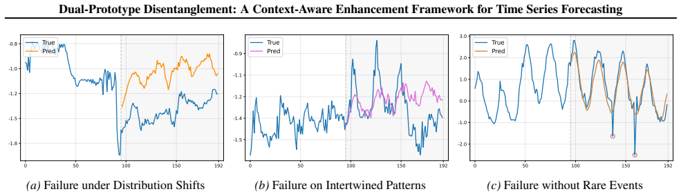
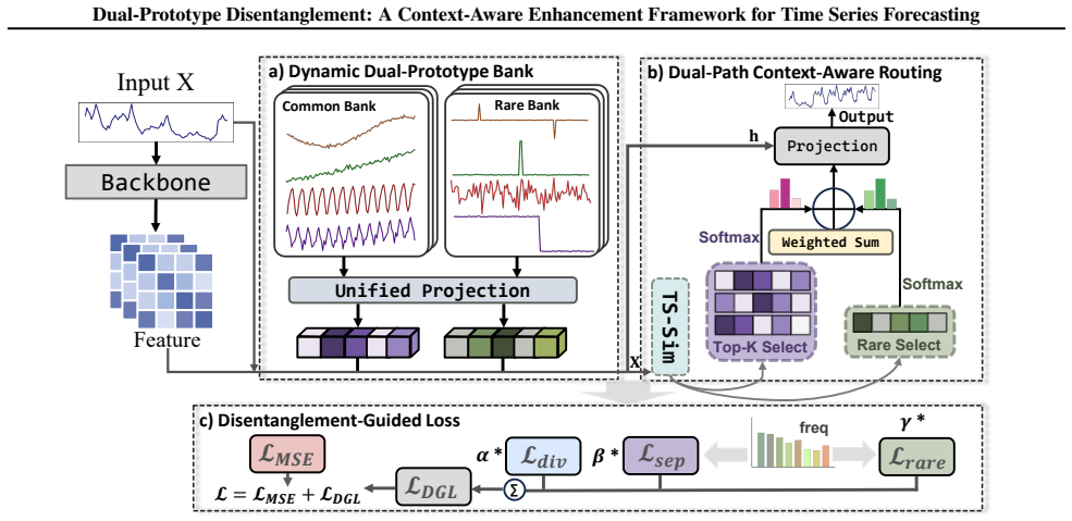
The central claim is that explicitly disentangling 'common' and 'rare' temporal patterns, and letting the model choose which pattern memory to consult based on the input context, improves forecasting on top of any strong backbone. Concretely, DPAD maintains a Dynamic Dual-Prototype bank: a common bank initialised from Gaussian-process priors over trend, seasonal and periodic shapes, and a rare bank starting from small random noise. A dual-path routing module scores each input window against both banks using Pearson correlation, retrieves the top common prototypes and at most one rare prototype, and fuses their weighted combination with the backbone's hidden representation. A disentanglement-
What carries the argument
The Dynamic Dual-Prototype Bank (DDP). Common prototypes are initialised as learnable sequences drawn from a mixture of Gaussian-process kernels (Linear + RBF + Periodic), encoding trend/seasonality priors; rare prototypes start as small-variance Gaussian noise. The Dual-Path Context-aware routing (DPC) projects the raw input into the same latent space, scores prototypes by Pearson correlation, selects top-K common prototypes and at most one rare prototype above a threshold, and produces a softmax-weighted fusion that is concatenated with the backbone hidden state to form the prediction. The Disentanglement-Guided Loss (DGLoss) adds a separation margin regulated by prototype activation frequ
Load-bearing premise
The framework assumes that every input window is usefully explained by either a common or a rare pattern class, and that a rare bank starting from random noise will memorise genuinely informative infrequent events instead of noise.
What would settle it
Take one benchmark where DPAD reports gains (for example, Electricity with iTransformer) and run the same protocol with the rare bank replaced by fixed random noise, or with rare events artificially removed from the training set; if the MSE improvement over the backbone largely persists, the rare-bank memorisation claimed by the paper is not what is driving the gain.
If this is right
- If the central claim holds, forecasting systems can be improved without redesigning their core architectures: DPAD is plug-and-play and adds less than 10% runtime and memory overhead for transformer and CNN backbones.
- The reported average MSE reductions (12.6% for DLinear, 9.3% for iTransformer) mean even lightweight baselines get a substantial accuracy boost.
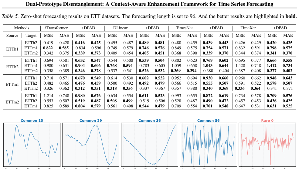
- The zero-shot results suggest that common and rare prototype memories learned on one set of datasets transfer to unseen datasets, which would be useful when target data are scarce.
- The ablation claims that using either bank alone yields marginal or negative gains implies both banks and their separation loss are jointly load-bearing, not just extra parameters.
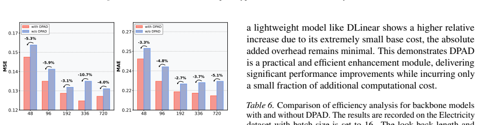
- Gains grow with look-back length (up to about 10.7% MSE reduction at length 720 on Electricity with TimeBridge), indicating the mechanism helps models use longer context rather than being overwhelmed by it.
Where Pith is reading between the lines
- The paper's bipartition of patterns into common and rare is a design choice; a continuous spectrum of rarity or multiple rarity levels might be a stronger model, and some of the reported gains could come from the extra capacity of the memory banks acting as a regulariser. This is my inference, not the paper's claim.
- Rare-bank sparsity (at most one rare prototype per window) could be tested against a top-k rare selection; if a single window contains several distinct rare deviations, the current design can represent only one of them.
- The Gaussian-process initialization of the common bank is not ablated against a random initialization; a direct comparison would isolate how much of the benefit comes from the prior versus the disentanglement objective.
- Because routing scores are Pearson correlations, the selected prototypes could double as an interpretability channel: monitoring which common or rare prototype fires could flag distribution shifts or anomalies during deployment.
Editorial analysis
A structured set of objections, weighed in public.
Referee Report
Summary. The paper proposes DPAD, a model-agnostic auxiliary framework for time series forecasting. It maintains a dual prototype bank (common patterns initialized with Gaussian-process kernels, rare patterns initialized with small Gaussian noise), uses a dual-path routing mechanism to retrieve and fuse prototypes with the backbone representation, and adds a disentanglement-guided loss (separation, rarity preservation, and diversity terms). The authors claim that plugging DPAD into five SOTA backbones yields consistent MSE/MAE improvements on long- and short-term benchmarks with negligible overhead, and they support this with main tables, ablations, zero-shot experiments, visualizations, and an efficiency analysis.
Significance. If the central claim were established, DPAD would be a practically valuable plug-in enhancement for forecasting, since it is model-agnostic and adds relatively few parameters. The paper includes full result tables, ablations of each component, zero-shot transfer experiments, and some efficiency measurements, which are commendable. However, the current evidence does not support the headline claim of 'consistent improvements': several baseline cells are implausibly weak, the aggregate statistics quoted in the main text are not reproducible from the appendix tables, and a number of backbone-dataset cells degrade under DPAD. These issues are load-bearing for the paper's main conclusion, so the manuscript cannot be accepted without substantive correction.
major comments (4)
- [§4.2, Table 1, Tables 9–10] The paper states that DPAD 'demonstrates consistent improvements across all backbone models' (Sec. 4.2). This is not supported by the full tables. Table 9 shows, e.g., TimesNet+DPAD on Exchange worsens from MSE 0.201 to 0.384 and on Electricity from 0.193 to 0.196; TimeXer+DPAD on ETTm2 worsens from 0.277 to 0.299; DLinear+DPAD on Exchange worsens from 0.338 to 0.345; Table 10 shows TimeBridge+DPAD on PEMS03 worsens from 0.153 to 0.155. The appendix itself (Sec. G.1) says only 'consistent improvements on most backbones and datasets,' a materially weaker claim. The abstract, introduction, and Sec. 4.2 should be qualified accordingly, and the systematic degradations should be discussed.
- [§4.2, Sec. G.1] The reported 'average MSE reduction of 9.3% for iTransformer' is not reproducible from Tables 9–10. Aggregating the 13 dataset averages in Table 1, the total MSE reduction is about 19.4%, the mean per-dataset reduction is about 10.8%, and the long-term-only mean reduction is about 1.7%. No standard aggregation yields 9.3%. The 12.6% figure for DLinear is similarly unexplained. The paper must either report a precise, reproducible aggregation rule or remove these headline percentages.
- [Table 10, PEMS04] The iTransformer baseline on PEMS04 (MSE 0.766, 0.799, 1.041, 1.045 for horizons 12/24/48/96; average 0.912) is implausibly weak. Published iTransformer results on PEMS04 are typically below 0.2 for these horizons, so this baseline is at least 5–10 times worse than expected and is very likely misconfigured. The corresponding +DPAD gain (0.912→0.199) is therefore not a reliable plug-in improvement. The same concern applies to the TimeBridge baseline on Traffic in Table 9 (1.411/1.427 vs. the much lower neighboring cells). These cells must be re-run with the official implementations and corrected configurations before any conclusion about PEMS or the average iTransformer improvement can be drawn.
- [§3.4, Eqs. (12)–(16), Fig. 3] The claimed 'disentanglement' is enforced by construction: L_sep, L_rare, and L_div explicitly push common and rare banks apart. The visualization in Fig. 3 therefore does not provide independent evidence that a natural common/rare dichotomy exists; it only verifies that the loss terms have their intended effect. More substantively, the framework's central assumption—that a binary common/rare split is the right organizing principle—is not tested against alternatives such as a continuous frequency spectrum or multiple rarity levels. Given that the gains in Tables 2–4 are small in absolute terms, the paper should address whether the improvement comes from the disentanglement mechanism or simply from the extra projection/routing parameters.
minor comments (6)
- [Eqs. (8)–(10)] When I_r = ∅ (no rare prototype passes the threshold), the definitions of ω_r and z_r in Eqs. (9)–(10) are undefined. The paper should specify a zero-vector fallback or otherwise handle the empty-rare-index case.
- [Sec. G.1, Table 10] The table header says PEMS03–PEMS06, but the rows and the dataset list (Table 7) use PEMS03, PEMS04, PEMS07, and PEMS08. Fix the header.
- [§4.5, Fig. 3] The text says the prototypes are visualized 'on the Weather dataset,' while the figure caption says 'on the Electricity dataset.' These should be aligned.
- [§4.1, §4.2] The text refers to 'seven real-world datasets' in Sec. 4.2, but Table 1 contains 13 dataset-backbone rows (9 long-term and 4 short-term). The count should be corrected.
- [Table 6] The efficiency analysis reports DLinear overhead of 57.1% in running time and 45.1% in memory. The text's statement that overhead is 'minimal' / 'negligible' should be qualified as 'small in absolute terms for large backbones, but large relative to lightweight backbones.'
- [Table 11] There are typographical inconsistencies in the full ablation table; for example, the Electricity 720 row lists +DPAD MAE 0.192, whereas the corresponding row in Table 9 reports MAE 0.289. The table needs careful proofreading.
Circularity Check
Forecasting gains are externally benchmarked and not circular; only the disentanglement visualization reduces to the model's own construction.
specific steps
-
self definitional
[Sec. 3.2 Eqs. (1)-(2), Sec. 3.4 Eq. (12), Sec. 4.5 Fig. 3]
"s_i^c ~ GP(0, λ_lK_l + λ_rK_r + λ_pK_p) ... s_j^r ~ N(0, σ^2 I) ... Lsep = E[ω·max(0, m−Δρ)+(1−ω)·max(0, m+Δρ)] ... In contrast, the rare bank displays markedly different characteristics, whose prototypes are characterized by abrupt, irregular fluctuations or sudden shifts."
The claimed evidence that DDP discovers a natural common/rare split is guaranteed by construction: common prototypes are initialized from smooth GP trend/seasonal kernels (Eq. 1), rare prototypes from white noise (Eq. 2), and Eq. (12) explicitly penalizes each bank for responding outside its assigned frequency regime. Observing smooth common and abrupt rare prototypes in Fig. 3 therefore restates the initialization plus the loss, not an independent empirical discovery. This does not affect the external forecasting comparisons, which are measured against unmodified backbones.
full rationale
The central claim—that DPAD improves MSE/MAE over five SOTA backbones—is an external empirical comparison against unmodified baselines and is not derivable from the DGLoss formula or the prototype initialization. The losses are optimization objectives, not fitted predictions. There is no load-bearing self-citation, no imported uniqueness theorem, and no ansatz smuggled in via citation. The one quasi-circular element is the prototype visualization in Sec. 4.5: because the common bank is initialized with smooth GP priors, the rare bank with Gaussian noise, and Lsep explicitly forces separation, the observed common-vs-rare contrast is a restatement of the construction rather than an independent discovery. That step is illustrative, not load-bearing for the forecasting gains. The suspicious PEMS04 iTransformer baseline and the unreproducible 9.3% average-reduction statistic are evidence/correctness concerns, not circularity under the definitions used here; they are therefore not reflected in the circularity score beyond noting that they weaken confidence in the empirical claim without making it circular.
Axiom & Free-Parameter Ledger
free parameters (6)
- M (number of common prototypes) =
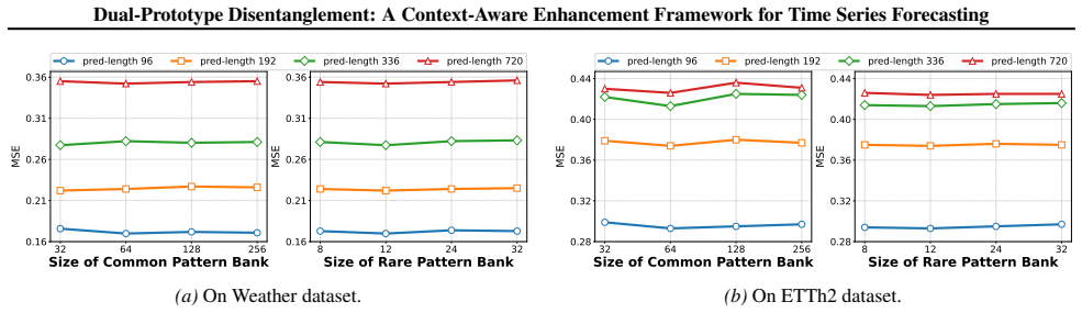
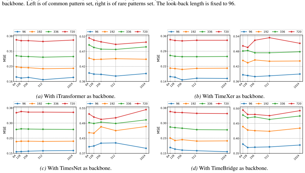
not specified; swept in 32–256
- N (number of rare prototypes) =
not specified; swept in 8–32
- λ_sep, λ_rare, λ_div (DGLoss weights) =
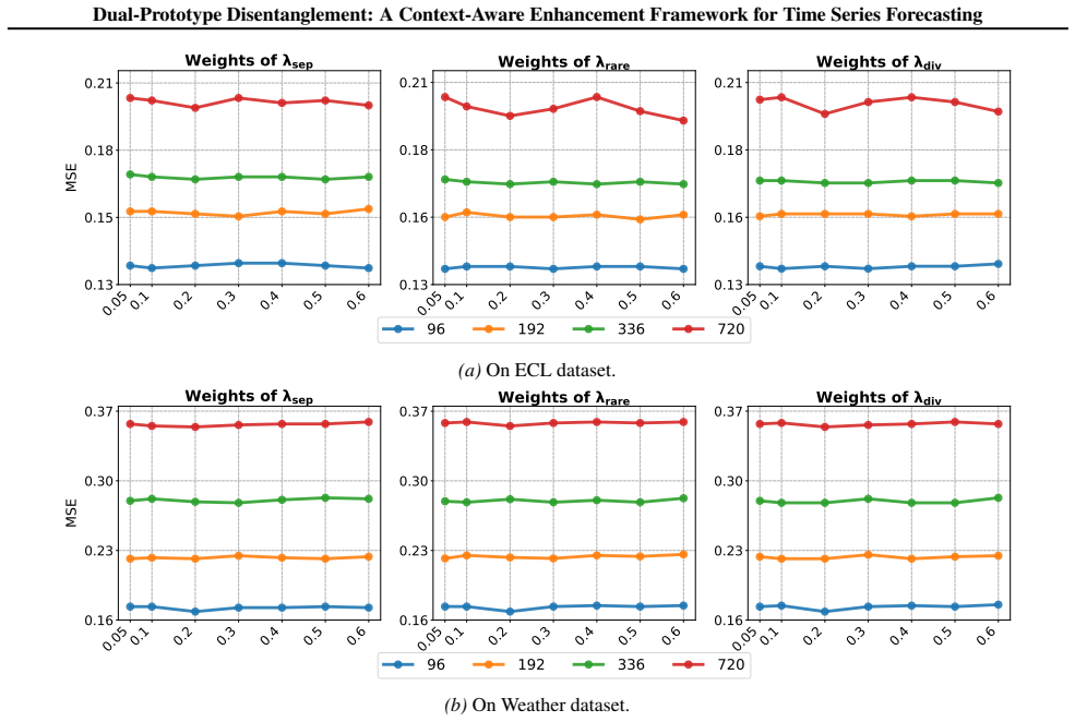
not specified; swept in 0.001–2.0
- τ (softmax temperature) and ε (rare-activation threshold) =
not specified
- GP kernel coefficients λl, λr, λp and kernel hyperparameters =
not specified
- Embedding/projection dimension D =
128 or 256 per case
axioms (4)
- ad hoc to paper The two-way common/rare dichotomy is sufficient to organize temporal patterns for forecasting
- ad hoc to paper GP-generated synthetic sequences provide a useful prior for common temporal patterns
- domain assumption Backbone baselines were correctly implemented and fairly tuned
- domain assumption Pearson correlation between projected input and prototypes is a valid scale-invariant matching score
invented entities (2)
-
Common Pattern Bank Bc
no independent evidence
-
Rare Pattern Bank Br
no independent evidence
read the original abstract
Real-world time series are governed by both recurring structures, such as trends and seasonality, and infrequent yet critical variations, such as abrupt shifts and rare events. However, existing methods often lack an explicit mechanism to organize and utilize these heterogeneous patterns according to their distinct forecasting roles. Consequently, common and rare patterns can become entangled, preventing models from dynamically distinguishing and selectively leveraging them according to context. To address this issue, we propose Dual-Prototype Adaptive Disentanglement (DPAD), a model-agnostic framework that organizes temporal patterns by their forecasting roles. Specifically, we construct a Dynamic Dual-Prototype bank (DDP), comprising a common pattern bank initialized with structured temporal priors to represent prevalent dynamics, and a rare bank that adaptively memorizes infrequent deviations. Then a Dual-Path Context-aware routing (DPC) mechanism enhances outputs with selectively retrieved context-specific pattern representations from DDP. A Disentanglement-Guided Loss (DGLoss) is further introduced to ensure that each prototype bank specializes in its designated role while maintaining sufficient coverage. Extensive experiments across diverse real-world benchmarks demonstrate that DPAD consistently improves the forecasting performance of a range of time-series models.
Figures
Reference graph
Works this paper leans on
-
[5]
Huang, S., Zhao, Z., Li, C., and Bai, L. Timekan: Kan- based frequency decomposition learning architecture for long-term time series forecasting.arXiv preprint arXiv:2502.06910,
-
[9]
Liu, P., Wu, B., Hu, Y ., Li, N., Dai, T., Bao, J., and tao Xia, S. Timebridge: Non-stationarity matters for long-term time series forecasting.arXiv preprint arXiv:2410.04442, 2025a. Liu, Y ., Hu, T., Zhang, H., Wu, H., Wang, S., Ma, L., and Long, M. itransformer: Inverted transformers are effective for time series forecasting.arXiv preprint arXiv:2310.06...
Pith/arXiv arXiv 2024
-
[10]
Liu, Z., Cheng, M., Zhao, G., Yang, J., Liu, Q., and Chen, E. Improving time series forecasting via instance-aware post- hoc revision.arXiv preprint arXiv:2505.23583, 2025b. Liu, Z., Yang, Z., Lin, X., Qiu, R., Wei, T., Zhu, Y ., Hamann, H., He, J., and Tong, H. Breaking silos: Adaptive model fusion unlocks better time series forecasting.arXiv preprint ar...
-
[11]
H., Sinthong, P., and Kalagnanam, J
Nie, Y ., Nguyen, N. H., Sinthong, P., and Kalagnanam, J. A time series is worth 64 words: Long-term forecasting with transformers. In11th International Conference on Learning Representations, ICLR 2023,
2023
-
[12]
Y ., Rasul, K., Schneider, A., Ma, L., Nevmyvaka, Y ., and Song, D
Ning, K., Pan, Z., Liu, Y ., Jiang, Y ., Zhang, J. Y ., Rasul, K., Schneider, A., Ma, L., Nevmyvaka, Y ., and Song, D. Ts-rag: Retrieval-augmented generation based time series foundation models are stronger zero-shot forecaster. arXiv preprint arXiv:2503.07649,
-
[13]
N., Carpov, D., Chapados, N., and Bengio, Y
Oreshkin, B. N., Carpov, D., Chapados, N., and Bengio, Y . N-beats: Neural basis expansion analysis for interpretable time series forecasting.arXiv preprint arXiv:1905.10437,
Pith/arXiv arXiv 1905
-
[14]
Qiu, X., Cheng, H., Wu, X., Hu, J., Guo, C., and Yang, B. A comprehensive survey of deep learning for multivariate time series forecasting: A channel strategy perspective. arXiv preprint arXiv:2502.10721, 2025a. Qiu, X., Wu, X., Cheng, H., Liu, X., Guo, C., Hu, J., and Yang, B. Dbloss: Decomposition-based loss function for time series forecasting.arXiv pr...
-
[15]
Shi, X., Wang, S., Nie, Y ., Li, D., Ye, Z., Wen, Q., and Jin, M. Time-moe: Billion-scale time series founda- tion models with mixture of experts.arXiv preprint arXiv:2409.16040,
-
[16]
Sun, Y ., Xie, Z., Chen, D., Eldele, E., and Hu, Q. Hier- archical classification auxiliary network for time series forecasting.arXiv preprint arXiv:2405.18975,
-
[17]
Tang, P. and Zhang, W. Unlocking the power of patch: Patch-based mlp for long-term time series forecasting. arXiv preprint arXiv:2405.13575,
-
[19]
Fredf: Learning to forecast in the frequency domain.arXiv preprint arXiv:2402.02399, 2025a
Wang, H., Pan, L., Chen, Z., Yang, D., Zhang, S., Yang, Y ., Liu, X., Li, H., and Tao, D. Fredf: Learning to forecast in the frequency domain.arXiv preprint arXiv:2402.02399, 2025a. Wang, S., Wu, H., Shi, X., Hu, T., Luo, H., Ma, L., Zhang, J. Y ., and Zhou, J. Timemixer: Decomposable multi- scale mixing for time series forecasting.arXiv preprint arXiv:24...
-
[20]
Timesnet: Temporal 2d-variation modeling for general time series analysis
Wu, H., Hu, T., Liu, Y ., Zhou, H., Wang, J., and Long, M. Timesnet: Temporal 2d-variation modeling for general time series analysis. In11th International Conference on Learning Representations, ICLR 2023, 2023a. Wu, H., Zhou, H., Long, M., and Wang, J. Interpretable weather forecasting for worldwide stations with a unified deep model.Nature Machine Intel...
Pith/arXiv arXiv 2023
-
[21]
Yu, X., Chen, Z., Ling, Y ., Dong, S., Liu, Z., and Lu, Y . Tem- poral data meets llm – explainable financial time series forecasting.arXiv preprint arXiv:2306.11025,
-
[22]
11 Dual-Prototype Disentanglement: A Context-Aware Enhancement Framework for Time Series Forecasting A. Datasets We conduct long-term forecasting experiments on 6 real-world datasets, including (1) ETT (ETTh1, ETTh2, ETTm1, ETTm2) contains 7 features of electricity transformer data from July 2016 to July 2018, which was sampled at hourly (ETTh1, ETTh2) an...
2016
-
[24]
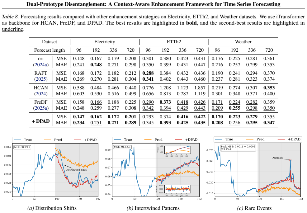
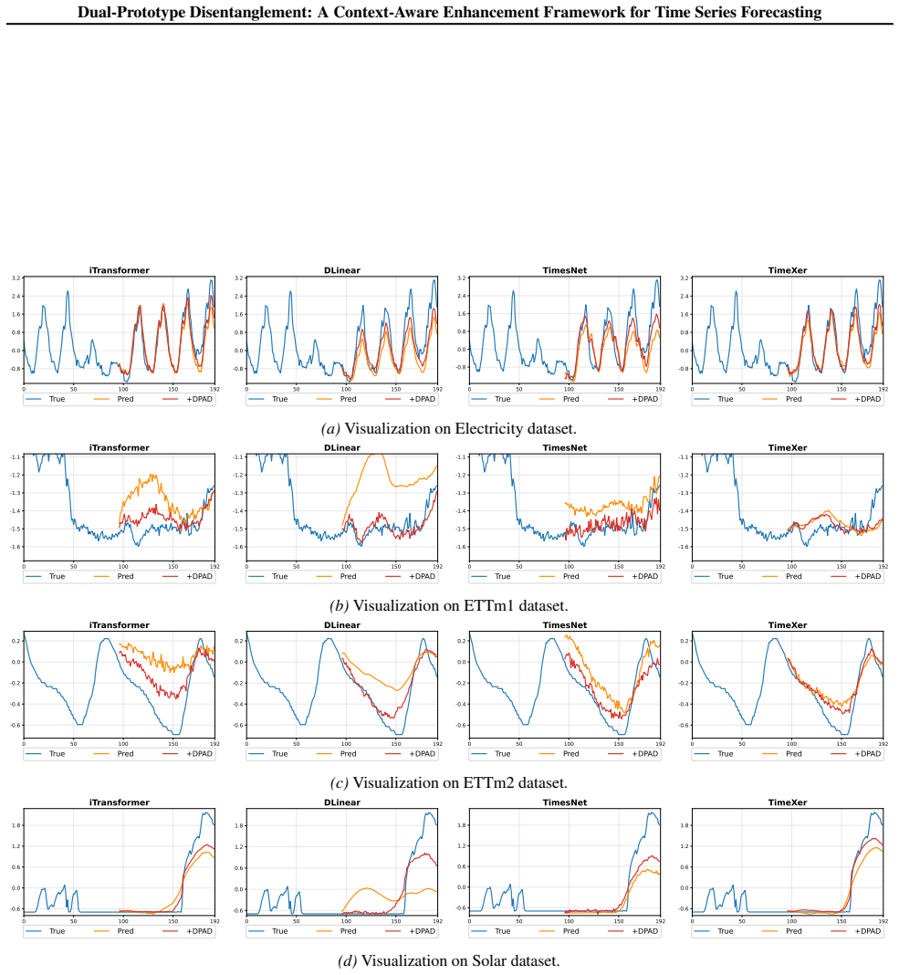
proposes a hierarchy-aware attention module supported by uncertainty-aware classifiers and a consistency loss to alleviate issues caused by the boundary effects during the classification of timesteps. FreDF (Wang et al., 2025a) bypasses the complexity of label autocorrelation by learning to forecast in the frequency domain. As shown in Table 8, DPAD consi...
arXiv 2025
-
[2010]
Bai, S., Kolter, J. Z., and Koltun, V . An empirical evalua- tion of generic convolutional and recurrent networks for sequence modeling.arXiv preprint arXiv:1803.01271,
-
[2014]
(4) Solar-Energy contains the solar power production of 137 PV plants in 2006, which is sampled every 10 minutes
(3) Exchange collects the daily exchange-rate data from eight different countries. (4) Solar-Energy contains the solar power production of 137 PV plants in 2006, which is sampled every 10 minutes. (5) Weather includes 21 meteorological factors collected every 10 minutes from the Max Planck Biogeochemistry Institute’s Weather Station in
2006
-
[2019]
Micn: Multi-scale local and global context modeling for long-term series forecasting
Wang, H., Peng, J., Huang, F., Wang, J., Chen, J., and Xiao, Y . Micn: Multi-scale local and global context modeling for long-term series forecasting. In11th International Conference on Learning Representations, ICLR 2023,
2023
-
[2020]
Han, S., Lee, S., Cha, M., Arik, S. O., and Yoon, J. Re- trieval augmented time series forecasting.arXiv preprint arXiv:2505.04163,
-
[2021]
Y ., Shi, X., Chen, P.-Y ., Liang, Y ., Li, Y .-F., Pan, S., and Wen, Q
Jin, M., Wang, S., Ma, L., Chu, Z., Zhang, J. Y ., Shi, X., Chen, P.-Y ., Liang, Y ., Li, Y .-F., Pan, S., and Wen, Q. Time-llm: Time series forecasting by reprogramming large language models.arXiv preprint arXiv:2310.01728,
-
[2022]
Patch-wise structural loss for time series forecasting.arXiv preprint arXiv:2503.00877,
Kudrat, D., Xie, Z., Sun, Y ., Jia, T., and Hu, Q. Patch-wise structural loss for time series forecasting.arXiv preprint arXiv:2503.00877,
-
[2023]
Pathformer: Multi-scale transform- ers with adaptive pathways for time series forecasting
Chen, P., Zhang, Y ., Cheng, Y ., Shu, Y ., Wang, Y ., Wen, Q., Yang, B., and Guo, C. Pathformer: Multi-scale transform- ers with adaptive pathways for time series forecasting. In 12th International Conference on Learning Representa- tions, ICLR 2024,
2024
-
[2024]
Reversible instance normalization for accurate time- series forecasting against distribution shift
Kim, T., Kim, J., Tae, Y ., Park, C., Choi, J.-H., and Choo, J. Reversible instance normalization for accurate time- series forecasting against distribution shift. In10th Inter- national Conference on Learning Representations, ICLR 2022,
2022
-
[2025]
Hu, Y ., Liu, P., Zhu, P., Cheng, D., and Dai, T. Adap- tive multi-scale decomposition framework for time series forecasting.arXiv preprint arXiv:2406.03751,
discussion (0)
Sign in with ORCID, Apple, or X to comment. Anyone can read and Pith papers without signing in.