REVIEW 4 major objections 5 minor 41 references
For QSVMs trained under local depolarising noise, the squared geometric margin — measured against the ideal kernel — is bounded above and below by explicit functions of the per-qubit noise survival probability (1−p)^{2N}, the clean margin,
Reviewed by Pith at T0; open to challenge. T0 means a machine referee read the full paper against a public rubric. the ladder, T0–T4 →
For QSVMs under local depolarising noise, the paper claims analytic upper and lower bounds on the squared geometric margin, validated (it says) by simulation and on an IBM device, plus empirical evidence that margins predict QSVM generalisation.
T0 review reviewed 2026-08-03 challenge →
load-bearing objection Kernel bound is real, but the margin bounds rest on an invalid quadratic-form step and a p=0 contradiction; salvageable but not acceptable as is. the 4 major comments →
The Cross-Kernel Margin: A Robustness Measure for Quantum Kernel Methods
The pith
A machine-rendered reading of the paper's core claim, the machinery that carries it, and where it could break.
The reading
Core claim
On the paper's own terms: local depolarising noise applied independently to each qubit degrades quantum kernel values by a contraction-plus-additive-constant form, K̃_ij ≤ (1−p)^{2LN}K_ij + (1−(1−p)^{2LN}). Substituting this bound into the SVM dual objective and using optimality relations for the soft-margin problem, the squared geometric margin of the noisy-trained, ideal-evaluated classifier satisfies γ̃² ≤ (1−p)^{2N}γ² / [2(1−mCγ²) − (1−p)^{2N}] and γ̃² ≥ γ²[1−2(1−p)^{2N}] / [2Cmγ² − 1], subject to feasibility constraints on mCγ². These are the upper and lower cross-kernel margin bounds; at p=0 the upper bound is tight. The construction also yields a hard-margin analogue and extends to L
What carries the argument
The central object is the cross-kernel margin: the squared geometric margin 1/∥w̃∥², where w̃ uses the dual solution obtained from the noisy kernel but the norm is evaluated against the ideal kernel. The carrying mechanism is the entrywise kernel bound derived from the Kraus decomposition of the local depolarising channel via Schatten/Hölder trace inequalities, together with the KKT identity Σ ᾱ_i y_i = 0, which is used to drop the additive constant when passing from kernel elements to the quadratic form ∥w̃∥² = Σ ᾱ_i ᾱ_j y_i y_j K̃_ij. SVM duality then converts the resulting inequalities into the margin bounds.
Load-bearing premise
The load-bearing premise is that the entrywise kernel bound can be multiplied by signed SVM weights and summed to bound the squared weight norm; the exact expression (89) shows a state-dependent signed remainder, and the lower bound's validity conditions contradict the p=0 equality unless they are stronger than stated.
What would settle it
Take any trained QSVM with 0 < Cmγ² < 1/2 and set p=0; the claimed lower bound (56) requires γ² ≥ γ²/(1−2Cmγ²), which is strictly stronger than the exact equality γ̃² = γ². A single such instance settles whether the validity conditions are sufficient. Separately, compute the weighted sum Σ_{i,j} ᾱ_i ᾱ_j y_i y_j [K̃_ij − (1−p)^{2N}K_ij − (1−(1−p)^{2N})] for a two-qubit dataset; any positive value violates the substitution step shared by both margin bounds.
If this is right
- Margin decay under local depolarising noise is controlled by the survival probability (1−p)^{2N}; increasing qubit number or encoding layers compounds the noise effect.
- The bounds give a computable range of regularisation parameters for which the noisy margin is guaranteed non-negative, allowing practitioners to certify training stability before running a noisy device.
- The noisy-trained, ideal-evaluated margin, not the self-consistent noisy margin, is the informative robustness statistic; the paper argues the latter hides noise-induced decay.
- In the noiseless setting, median geometric margin can serve as a proxy for QSVM generalisation, with Pearson correlations above 0.9 across the tested datasets.
- Global depolarising noise models understate performance loss; local per-qubit noise should be preferred when modelling QSVM robustness in the NISQ era.
Where Pith is reading between the lines
- A tighter, state-dependent bound could replace the additive constant: the paper's exact expression (89) exhibits a signed remainder depending on the purity and Pauli coefficients of the data states, so the loose entrywise bound may be far from tight for low-purity states.
- The label-corruption experiments establish margin–accuracy correlation in the ideal setting; applying the same corruption pipeline under kernel noise would test whether the cross-kernel margin predicts accuracy under device noise as directly as it does under label noise.
- The bounds suggest an experimentally testable noise threshold: solving for the p at which the lower bound crosses zero should predict where QSVM test accuracy collapses, and that prediction can be checked on hardware.
- The derivation structure should carry to other single-qubit noise channels, such as amplitude damping, by replacing (1−p)^{2N} with the channel-dependent survival factor; disagreement would show where the depolarising assumption is load-bearing.
Editorial analysis
A structured set of objections, weighed in public.
Referee Report
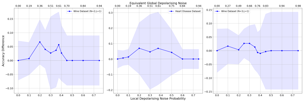
Summary. The paper proposes a margin-based robustness measure for quantum kernel-assisted support vector machines (QSVMs) under local depolarising noise. It derives an entrywise upper bound on noisy kernel elements, then uses SVM KKT and optimality relations to obtain upper and lower bounds on the squared geometric margin of a QSVM trained on the noisy kernel and evaluated against the ideal kernel. The main theoretical results are eqs. (42) and (56). The paper also reports empirical margin-accuracy correlations across several datasets, a comparison of local vs. global depolarising noise, and an experiment on the IBM ibm_fez device.
Significance. If the main theorem were correct, it would be a valuable analytic characterisation of noise-induced margin decay for QSVMs under a realistic, per-qubit noise model, and it would strengthen the case for margin-based generalisation analysis in quantum machine learning. The entrywise kernel bound (33) is a genuine and checkable derivation, and the empirical correlation between median geometric margin and test accuracy (r > 0.9) is interesting. However, the central step that converts the entrywise kernel bound into a quadratic-form bound is invalid, and the lower margin bound is contradicted already at p=0. The theoretical contribution is therefore not established; the useful empirical observations do not rescue the main claim.
major comments (4)
- [Appendix A.3.1/A.3.2, eqs. (91)-(95)] The substitution of the entrywise bound K̃_ij ≤ A K_ij + B into the quadratic form is invalid because the coefficients s_i s_j = α_i α_j y_i y_j are not nonnegative. The KKT condition Σα_i y_i=0 removes only the BΣs_i s_j term; it does not control the A term. Concrete counterexample: N=2, L=1, p=0.1, training states |00⟩ and |11⟩ with labels ±1. For the local depolarising channel λ=1−4p/3=0.8667, K̃_11=K̃_22=((1+λ²)/2)²≈0.766, K̃_12=((1−λ²)/2)²≈0.0155, and A=(0.9)^4≈0.656. For the two-point SVM, the optimal noisy dual solution (for C not saturated) is v=α(1,−1) with α=2/(K̃_11+K̃_22−2K̃_12). Then v^T K̃ v ≈ 2.665 while A v^T K v ≈ 2.330, so v^T K̃ v > A v^T K v. This contradicts (93). Since (93) is used to derive (41) and (55), the margin bounds (42) and (56) are unsupported.
- [Section 6.3, eq. (56) and conditions (57)–(61)] At p=0 the noisy kernel coincides with the clean kernel, so the noisy margin equals the clean margin: γ̃²_α = γ²_α. Under condition (61), which is allowed when Cmγ²_α < 1/2, the right-hand side of (56) becomes γ²_α / (1 − 2Cmγ²_α) > γ²_α. Thus (56) asserts γ²_α ≥ γ²_α / (1 − 2Cmγ²_α) > γ²_α, a direct contradiction. This failure is independent of the Result 1A/1B issue and shows that the lower margin bound is false in an allowed parameter regime, not merely unproven.
- [Appendix A.2, eq. (89)] Equation (89) is called the exact expression for the noisy kernel, but the remainder sum is restricted to m=n≠0. The m≠n terms are not shown to vanish; nothing in the derivation up to (87) eliminates them, and the original sum in (76) contains no such restriction. The label 'exact' is therefore unjustified, and (89) cannot serve as a repair for the signed-remainder problem that invalidates the quadratic-form step in Results 1A/1B.
- [Section 7.1 and eqs. (47)–(49)] The feasible C′ range used in the numerical validation is not fully a priori: C′_min in (49) contains the noisy margin γ̃², the quantity being bounded. The paper estimates it on a held-out validation set and then selects datasets that have an overlapping feasible C′ range across noise levels. Although the authors acknowledge this, it means the agreement in Figs. 11–13 is a weaker test of the theory than a parameter-free bound would provide, and the dataset-selection step conditions the empirical evidence.
minor comments (5)
- [Section 3.3, eqs. (12)–(15)] The notation for the noise probability changes from p′_L to p_L to p without an explicit statement of the relation. In particular, p in (15) should be p_L, and the domain p_L∈[0,3/4] should be stated where the Kraus operators are introduced.
- [Eqs. (46)–(49) and Eq. (63)] The symbol C′ is first defined as mC before eq. (46) and later as C_0 m^{1−β} in eq. (63). These are different objects; please use distinct notation or explicitly state the reparametrization.
- [Appendix A.2, eq. (83)] The definition of c_{n_i} in Appendix A.2 conflicts with the c_{αβ} product constants used in Section 6.1. This makes the derivation hard to follow; distinct symbols would help.
- [Section 7.2, Fig. 13] The statement that the hardware noise level is 'within the particular noise range' is not quantified. The crossing points of the green horizontal line with the bounds are used to infer a noise level, but no uncertainty or error bar for the hardware margin is given.
- [General] The arXiv title mentions a 'cross-kernel margin', but the term is not defined in the manuscript. Either define this quantity explicitly or adjust the title to match the content.
Circularity Check
The margin-bound derivation does not assume its target, but the numerical validation is partly circular: C'_min is computed from the noisy margin it is supposed to bound.
specific steps
-
fitted input called prediction
[Section 6.2, eqs. (47)-(49); Section 7.1, Dataset Selection]
"Notably, the expression for the minimum C ′ value contains the noisy margin, i.e. the quantity that we want to bound. ... In our numerical experiments, a closer estimate for the value of C ′ min is obtained by computing an estimate noisy margin on a separate, held-out validation set. This value is used in the C ′ min calculation and consistently provides a tighter estimate of the minimum value."
The upper-bound test chooses C' inside [C'_min, C'_max), but C'_min is algebraically obtained by rearranging the target upper bound and explicitly contains the noisy margin γ̃² (eqs. 47-49). Using a validation-set estimate of γ̃² to compute C'_min means the chosen C' is, by construction, one for which the bound is satisfied for that estimate. The plotted 'theoretical upper bound' is therefore calibrated to the very quantity it is supposed to constrain, so the empirical confirmation is partly forced. The theorem derivation itself does not use this estimate; hence this is validation-side circularity rather than a definitional circularity of the bound.
full rationale
Walking the claimed derivation chain: the kernel-element bound (33) is derived from depolarising-channel trace inequalities and does not assume the margin result. Results 1A/1B attempt to pass from this entrywise kernel bound to a quadratic-form norm bound; whether or not that step is mathematically valid, it is not circular because it does not posit the target inequality. The final margin bounds then follow from SVM optimality and KKT relations rather than from the empirical quantities they bound. There is no load-bearing self-citation: the only author self-citation is introductory and not used to justify the central derivation. The one genuine circular element is in the validation protocol: C'_min in eqs. (47)-(49) contains the noisy margin, and Section 7.1 explicitly uses a validation-set estimate of that noisy margin to compute C'_min, so the C' used to draw the 'theoretical' bound is selected from a range defined by the quantity the bound is meant to constrain. The false quadratic-form substitution in Results 1A/1B and the p=0 contradiction in lower-bound condition (61) are serious correctness problems, but they are proof failures rather than cases where the output is equivalent to the input by construction, so they do not further raise the circularity score.
Axiom & Free-Parameter Ledger
free parameters (3)
- β (regularisation scaling exponent) =
β=0 (Heart, Gaussian); β=1 (Breast Cancer, Wine)
- C₀ (initial SVM regularisation parameter) =
10 (Heart), 100 (Gaussian), 1000 (Breast Cancer, Wine)
- feasible C′ window =
[0,21.1), [32.4,112.6), [0,544.7), [0,38.9), [0.6,125)
axioms (6)
- standard math SVM dual and primal optimality: L(α,K̃) ≤ L(ᾱ,K̃) and P(wα,·) ≤ P(wᾱ,·); KKT conditions including Σαᵢyᵢ=0 and αᵢ=C for ξᵢ≠0
- standard math Trace/Hölder/Schatten-norm inequalities and purity bound Tr(ρ²) ≤ 1 used to bound each noisy trace term by 1
- domain assumption Local depolarising channel model (Kraus form, eq 15) applied independently to each qubit after each unitary layer
- domain assumption Survival-probability matching p_GS=(1−p_G)^L versus p_LS=(1−p_L)^{NL} as the fair basis for comparing global and local noise
- domain assumption IQP feature map plus Hilbert-Schmidt kernel K(xᵢ,xⱼ)=Tr(ρ(xᵢ)ρ(xⱼ)) after PCA to 2–3 features
- ad hoc to paper Unproven matrix inequality: the entrywise kernel bound K̃ ≤ AK + BJ implies the quadratic-form bound sᵀK̃s ≤ A sᵀKs for s = ᾱ∘y
invented entities (1)
-
Noisy geometric margin γ̃² (margin of the dual solution trained on the noisy kernel, evaluated against the ideal kernel)
independent evidence
Cite this review
Pith. "Pith review of The Cross-Kernel Margin: A Robustness Measure for Quantum Kernel Methods." pith.science (2026). https://pith.science/paper/ZDTII2MJ
@misc{pith2026260123084,
  author       = {Pith},
  title        = {Pith review of: The Cross-Kernel Margin: A Robustness Measure for Quantum Kernel Methods},
  year         = {2026},
  howpublished = {\url{https://pith.science/paper/ZDTII2MJ}},
  note         = {Machine review of arXiv:2601.23084}
}
read the original abstract
Quantum devices in the current Noisy Intermediate-Scale Quantum (NISQ) era are inherently affected by noise, which can degrade the predictive performance of quantum machine learning models. In this work, we introduce a new margin-based robustness measure for Quantum Kernel-Assisted Support Vector Machines (QSVMs), termed the cross-kernel margin. This measure quantifies the stability of a classifier learned under a perturbed kernel relative to the ideal feature space. We derive a posteriori stability bounds for the corresponding cross-kernel inverse squared-margin under kernel perturbations using the Tikhonov-stabilised SVM dual formulation. The local depolarising noise model is then applied to this framework to induce perturbations in the kernel. The resulting bounds are numerically checked using simulations across multiple datasets and further tested using kernel matrices obtained from real quantum hardware and a noisy backend simulator. Furthermore, we empirically compare the degradation of test accuracy under local depolarising noise with the commonly used global depolarising noise model in order to motivate its use in our study. Finally, we present empirical results linking margin-based quantities with the generalisation performance of QSVMs, providing additional motivation for our margin-based robustness analysis.
Figures




Reference graph
Works this paper leans on
-
[1]
An introduction to quantum machine learning.Contemporary Physics, 56(2):172–185, 2015
Maria Schuld, Ilya Sinayskiy, and Francesco Petruccione. An introduction to quantum machine learning.Contemporary Physics, 56(2):172–185, 2015
2015
-
[2]
Pac-bayes & margins.Advances in neural information pro- cessing systems, 15, 2002
John Langford and John Shawe-Taylor. Pac-bayes & margins.Advances in neural information pro- cessing systems, 15, 2002
2002
-
[3]
A pac-bayesian margin bound for linear classifiers: Why svms work.Advances in neural information processing systems, 13, 2000
Ralf Herbrich and Thore Graepel. A pac-bayesian margin bound for linear classifiers: Why svms work.Advances in neural information processing systems, 13, 2000
2000
-
[4]
Simplified pac-bayesian margin bounds
David McAllester. Simplified pac-bayesian margin bounds. InLearning Theory and Kernel Machines: 16th Annual Conference on Learning Theory and 7th Kernel Workshop, COLT/Kernel 2003, Wash- ington, DC, USA, August 24-27, 2003. Proceed- ings, pages 203–215. Springer, 2003
2003
-
[5]
Afshin Rostamizadeh Mehryar Mohri and Ameet Talwalkar.Foundations of Machine Learning, 2nd ed.MIT Press, 2018
2018
-
[6]
Near-tight margin-based generalization bounds for support vector machines
Allan Grønlund, Lior Kamma, and Kasper Green Larsen. Near-tight margin-based generalization bounds for support vector machines. InInter- national Conference on Machine Learning, pages 3779–3788. PMLR, 2020
2020
-
[7]
Generaliza- tion performance of support vector machines and other pattern classifiers.Advances in Kernel meth- ods—support vector learning, pages 43–54, 1999
Peter Bartlett and John Shawe-Taylor. Generaliza- tion performance of support vector machines and other pattern classifiers.Advances in Kernel meth- ods—support vector learning, pages 43–54, 1999
1999
-
[8]
On the uniform convergence of relative frequencies of events to their probabilities
Vladimir Vapnik. On the uniform convergence of relative frequencies of events to their probabilities. InDoklady Akademii Nauk USSR, volume 181, pages 781–787, 1968
1968
-
[9]
Bounds on error expectation for support vector machines
Vladimir Vapnik and Olivier Chapelle. Bounds on error expectation for support vector machines. Neural computation, 12(9):2013–2036, 2000
2013
-
[10]
Springer Science & Business Media, 2006
Vladimir Vapnik.Estimation of dependences based on empirical data. Springer Science & Business Media, 2006
2006
-
[11]
Support- vector networks.Machine learning, 20(3):273– 297, 1995
Corinna Cortes and Vladimir Vapnik. Support- vector networks.Machine learning, 20(3):273– 297, 1995
1995
-
[12]
Quantum computing in the nisq era and beyond.Quantum, 2:79, 2018
John Preskill. Quantum computing in the nisq era and beyond.Quantum, 2:79, 2018
2018
-
[13]
Generalization in quantum machine learning from few training data.Nature communications, 13(1):4919, 2022
Matthias C Caro, Hsin-Yuan Huang, Marco Cerezo, Kunal Sharma, Andrew Sornborger, Lukasz Cincio, and Patrick J Coles. Generalization in quantum machine learning from few training data.Nature communications, 13(1):4919, 2022
2022
-
[14]
Understanding quantum machine learn- ing also requires rethinking generalization.Nature Communications, 15(1):2277, 2024
Elies Gil-Fuster, Jens Eisert, and Carlos Bravo- Prieto. Understanding quantum machine learn- ing also requires rethinking generalization.Nature Communications, 15(1):2277, 2024
2024
-
[15]
Understanding gen- eralization in quantum machine learning with mar- gins
Tak Hur and Daniel K Park. Understanding gen- eralization in quantum machine learning with mar- gins. InForty-second International Conference on Machine Learning, 2024
2024
-
[16]
Towards understanding the power of quantum kernels in the nisq era.Quantum, 5: 531, 2021
Xinbiao Wang, Yuxuan Du, Y ong Luo, and Dacheng Tao. Towards understanding the power of quantum kernels in the nisq era.Quantum, 5: 531, 2021
2021
-
[17]
Power characterization of noisy quan- tum kernels.IEEE Transactions on Neural Net- works and Learning Systems, 2025
Y abo Wang, Bo Qi, Xin Wang, Tongliang Liu, and Daoyi Dong. Power characterization of noisy quan- tum kernels.IEEE Transactions on Neural Net- works and Learning Systems, 2025
2025
-
[18]
Generalization error bound for quantum machine learning in nisq era—a survey.Quantum Machine Intelligence, 6(2):90, 2024
Bikram Khanal, Pablo Rivas, Arun Sanjel, Korn Sooksatra, Ernesto Quevedo, and Alejandro Ro- driguez. Generalization error bound for quantum machine learning in nisq era—a survey.Quantum Machine Intelligence, 6(2):90, 2024
2024
-
[19]
Cambridge university press, 2010
Michael A Nielsen and Isaac L Chuang.Quantum computation and quantum information. Cambridge university press, 2010. 22
2010
-
[20]
Rademacher and gaussian complexities: Risk bounds and structural results.Journal of Machine Learning Research, 3(Nov):463–482, 2002
Peter L Bartlett and Shahar Mendelson. Rademacher and gaussian complexities: Risk bounds and structural results.Journal of Machine Learning Research, 3(Nov):463–482, 2002
2002
-
[21]
Pseudo- dimension of quantum circuits.Quantum Machine Intelligence, 2(2):14, 2020
Matthias C Caro and Ishaun Datta. Pseudo- dimension of quantum circuits.Quantum Machine Intelligence, 2(2):14, 2020
2020
-
[22]
Generalization in quantum machine learn- ing: A quantum information standpoint.PRX Quan- tum, 2(4):040321, 2021
Leonardo Banchi, Jason Pereira, and Stefano Pi- randola. Generalization in quantum machine learn- ing: A quantum information standpoint.PRX Quan- tum, 2(4):040321, 2021
2021
-
[23]
Tobias Haug and M. S. Kim. Generalization of quantum machine learning models using quan- tum fisher information metric.Phys. Rev. Lett., 133:050603, Jul 2024. doi:10.1103/PhysRevLett. 133.050603. URLhttps://link.aps.org/doi/10. 1103/PhysRevLett.133.050603
-
[24]
Statistical complexity of quan- tum circuits.Physical Review A, 105(6):062431, 2022
Kaifeng Bu, Dax Enshan Koh, Lu Li, Qingxian Luo, and Y aobo Zhang. Statistical complexity of quan- tum circuits.Physical Review A, 105(6):062431, 2022
2022
-
[25]
Effects of quantum resources and noise on the statistical complexity of quantum circuits.Quantum Science and Technology, 8(2): 025013, 2023
Kaifeng Bu, Dax Enshan Koh, Lu Li, Qingxian Luo, and Y aobo Zhang. Effects of quantum resources and noise on the statistical complexity of quantum circuits.Quantum Science and Technology, 8(2): 025013, 2023
2023
-
[26]
Rademacher com- plexity of noisy quantum circuits.arXiv preprint arXiv:2103.03139, 2021
Kaifeng Bu, Dax Enshan Koh, Lu Li, Qingx- ian Luo, and Y aobo Zhang. Rademacher com- plexity of noisy quantum circuits.arXiv preprint arXiv:2103.03139, 2021
Pith/arXiv arXiv 2021
-
[27]
Understanding deep learning (still) requires rethinking generaliza- tion.Communications of the ACM, 64(3):107–115, 2021
Chiyuan Zhang, Samy Bengio, Moritz Hardt, Ben- jamin Recht, and Oriol Vinyals. Understanding deep learning (still) requires rethinking generaliza- tion.Communications of the ACM, 64(3):107–115, 2021
2021
-
[28]
Spectrally-normalized margin bounds for neural networks.Advances in neural information processing systems, 30, 2017
Peter L Bartlett, Dylan J Foster, and Matus J Tel- garsky. Spectrally-normalized margin bounds for neural networks.Advances in neural information processing systems, 30, 2017
2017
-
[29]
Exponential concentration in quantum kernel methods.Nature communications, 15(1):5200, 2024
Supanut Thanasilp, Samson Wang, Marco Cerezo, and Zoë Holmes. Exponential concentration in quantum kernel methods.Nature communications, 15(1):5200, 2024
2024
-
[30]
A training algorithm for optimal margin classifiers
Bernhard E Boser, Isabelle M Guyon, and Vladimir N Vapnik. A training algorithm for optimal margin classifiers. InProceedings of the fifth an- nual workshop on Computational learning theory, pages 144–152, 1992
1992
-
[31]
Quantum ma- chine learning in feature hilbert spaces.Physical review letters, 122(4):040504, 2019
Maria Schuld and Nathan Killoran. Quantum ma- chine learning in feature hilbert spaces.Physical review letters, 122(4):040504, 2019
2019
-
[32]
Robert J Lyon, BW Stappers, Sally Cooper, John Martin Brooke, and Joshua D Knowles. Fifty years of pulsar candidate selection: from simple fil- ters to a new principled real-time classification ap- proach.Monthly Notices of the Royal Astronomical Society, 459(1):1104–1123, 2016
2016
-
[33]
Supervised learning with quantum-enhanced feature spaces
Vojt ˇech Havlí ˇcek, Antonio D Córcoles, Kristan Temme, Aram W Harrow, Abhinav Kandala, Jerry M Chow, and Jay M Gambetta. Supervised learning with quantum-enhanced feature spaces. Nature, 567(7747):209–212, 2019
2019
-
[34]
Cross-validation., 2019
Daniel Berrar et al. Cross-validation., 2019
2019
-
[35]
Principal component analysis.Chemometrics and intelligent laboratory systems, 2(1-3):37–52, 1987
Svante Wold, Kim Esbensen, and Paul Geladi. Principal component analysis.Chemometrics and intelligent laboratory systems, 2(1-3):37–52, 1987
1987
-
[36]
Learnability of quan- tum neural networks.PRX quantum, 2(4):040337, 2021
Yuxuan Du, Min-Hsiu Hsieh, Tongliang Liu, Shan Y ou, and Dacheng Tao. Learnability of quan- tum neural networks.PRX quantum, 2(4):040337, 2021
2021
-
[37]
K-fold cross validation for error rate estimate in support vector machines
Davide Anguita, Alessandro Ghio, Sandro Ridella, and Dario Sterpi. K-fold cross validation for error rate estimate in support vector machines. InDMIN, pages 291–297, 2009
2009
-
[38]
Ville Bergholm, Josh Izaac, Maria Schuld, Chris- tian Gogolin, Shahnawaz Ahmed, Vishnu Ajith, M Sohaib Alam, Guillermo Alonso-Linaje, B Akash- Narayanan, Ali Asadi, et al. Pennylane: Automatic differentiation of hybrid quantum-classical compu- tations.arXiv preprint arXiv:1811.04968, 2018. 23
Pith/arXiv arXiv 2018
-
[39]
Wood, Jake Lishman, Julien Gacon, Simon Martiel, Paul D
Ali Javadi-Abhari, Matthew Treinish, Kevin Krsulich, Christopher J. Wood, Jake Lishman, Julien Gacon, Simon Martiel, Paul D. Nation, Lev S. Bishop, An- drew W. Cross, Blake R. Johnson, and Jay M. Gambetta. Quantum computing with Qiskit, 2024
2024
-
[40]
com/, 2025
IBM Quantum.https://quantum.cloud.ibm. com/, 2025
2025
-
[41]
M" or "B
Kolby Nottingham Markelle Kelly, Rachel Longjohn. The uci machine learning repository.https:// archive.ics.uci.edu, 1987. 24 A Appendix A.1 Kernel Bound (LLayers) In this section, we present bounds for the case of ker- nel elements affected byLapplications of a local depo- larising noise channel for anN-qubit system. Before we rework our bound to includeL...
1987
This paper was first reviewed by deepseek-v4-flash on August 3, 2026.
discussion (0)
Sign in with ORCID, Apple, or X to comment. Anyone can read and Pith papers without signing in.