REVIEW 4 major objections 5 minor 17 references
Vision transformers finetune best when the components that react most strongly to input changes — attention modules and the first feedforward layer — are the ones updated, not the smooth LayerNorms.
Reviewed by Pith at T0; open to challenge. T0 means a machine referee read the full paper against a public rubric. the ladder, T0–T4 →
T0 review · deepseek-v4-flash
2026-08-03 03:44 UTC pith:C43B7LBA
load-bearing objection The plasticity measure is a cheap, sensible criterion for choosing ViT components to finetune, and the empirical study is thorough, but the headline comparison conflates plasticity with parameter count, so the causal claim is currently overstated. the 4 major comments →
Vision Transformer Finetuning Benefits from Non-Smooth Components
The pith
A machine-rendered reading of the paper's core claim, the machinery that carries it, and where it could break.
Core claim
The central claim is that the plasticity of a transformer component, defined as the expected ratio of output change to input change, predicts how much that component benefits from finetuning. The authors prove that this plasticity is bounded above by the Lipschitz constant, and they derive explicit upper bounds for LayerNorm, feedforward layers, and multi-head self-attention under bounded-token assumptions. Comparing these bounds yields the theoretical ranking MHA > FC1 ≈ FC2 > LN2 ≈ LN1. Empirical measurements on an ImageNet-pretrained ViT-Base and ViT-Huge confirm this order, with attention and feedforward modules having plasticity greater than 1 and LayerNorms below 1. In isolated finetun
What carries the argument
The central object is the plasticity measure P(f) = E[||f(x)-f(y)||_F / ||x-y||_F], the average rate of change over pairs of token sequences. Because P(f) ≤ Lip(f), it quantifies the average sensitivity of a module to input perturbations, with high plasticity implying low smoothness. The theoretical ranking comes from upper bounds on P(f): LayerNorm's bound is (1/σ)||γ||∞, feedforward linear layers are bounded by the spectral norm of their weight matrix, and multi-head self-attention is bounded by a sum over heads of ||O_h|| ||V_h|| (√(3n + (12n+3)r^4||A_h||^2)), with a tighter variant √n + α²E||A_h|| under image-energy assumptions. These bounds place attention above the feedforward layers,
Load-bearing premise
The empirical comparison assumes that, after sweeping learning rates, the 28M-parameter attention/feedforward configurations and the 18K-parameter LayerNorm configurations are fairly comparable, i.e., parameter count is not the true driver of the finetuning gap. This enters at Section 5.2/Table 3, where MHA/FC1/FC2 each update about 33% of ViT-Base while LN1/LN2 update 0.02%; if capacity explains the accuracy differences, the plasticity ranking is a correlate rather than a ca
What would settle it
Multiply the LayerNorm weight vector gamma by a constant on a pretrained ViT so that its measured plasticity matches that of the feedforward layer, while keeping the number of trainable parameters at 18K. If finetuning this high-plasticity LayerNorm still does not approach the accuracy of the feedforward configurations, then parameter count, not plasticity, explains the observed gap. Conversely, if it does, the plasticity ranking is confirmed as a causal driver.
If this is right
- Selective finetuning of a ViT should update the attention modules and the first feedforward linear layer, not the LayerNorm layers, to get better and more stable accuracy.
- Finetuning high-plasticity components reduces the sensitivity to learning rate and initialization, so the choice of component can shrink the hyperparameter search space.
- The plasticity ranking is consistent over 11 classification benchmarks and holds for both ViT-Base and ViT-Huge, indicating it is an intrinsic property of the pretrained components.
- Because the ranking is known before finetuning, it can guide the design of parameter-efficient adaptation methods that update only the most adaptive modules.
Where Pith is reading between the lines
- The plasticity measure can be computed from the pretrained model alone, so it could serve as a cheap pre-finetuning criterion for choosing which components to adapt, potentially avoiding exhaustive search over module combinations.
- The assumption that image tokens in a given position share a mean and standard deviation, used for the LayerNorm bound, is natural for normalized images but may not transfer to text or time-series inputs; similar proofs would be needed for other modalities.
- The authors' finding that high plasticity aids finetuning stands in tension with the common practice of regularizing smoothness (e.g., through Lipschitz constraints) — a direct test would compare finetuning under a Lipschitz penalty on the attention module versus on the feedforward layer.
- A concrete extension consistent with the paper's own future-work remarks would be to apply low-rank adaptation (LoRA-style) only to the high-plasticity modules and measure whether the improved finetuning persists with far fewer trainable parameters.
Editorial analysis
A structured set of objections, weighed in public.
Referee Report
Summary. The paper introduces a measure of transformer-component 'plasticity' (Definition 1) as the average rate of change of a module's output with respect to its input, and argues that high plasticity (low smoothness) is beneficial for finetuning. The authors derive upper bounds on this quantity for LayerNorm, feedforward layers, and multi-head self-attention (Propositions 1–4), use these to propose a theoretical ranking (Takeaway 1), refine it empirically on ViT-Base and ViT-Huge (Takeaway 2: MHA→FC1→FC2→LN2→LN1), and then finetune each component in isolation on 11 classification benchmarks. They report that components with higher plasticity yield better and more stable finetuning accuracy, and conclude that practitioners should prioritize attention and the first feedforward layer during adaptation (Takeaway 3).
Significance. If the causal claim in Takeaway 3 holds, the paper would provide a simple, theoretically motivated criterion for selecting finetuning components, potentially replacing exhaustive search. The paper is strong in its breadth: over 1,000 finetuning runs (approximately 800 in the main text; see minor comment), multiple benchmarks, two model sizes, and publicly available code. The empirical plasticity ranking is consistent across benchmarks and model sizes, and the within-group finetuning comparisons (MHA vs. FC1 vs. FC2, and LN1 vs. LN2) are useful evidence. However, the central cross-group conclusion is currently undermined by a parameter-count confound, and the formal definition of plasticity is not well-posed as stated. These issues are fixable, but they are load-bearing.
major comments (4)
- [Section 3, Definition 1] The definition of P(f) invokes 'the uniform distribution over the set of distinct pairs of sequences of tokens in (R^d)^n'. No uniform probability measure exists on this unbounded, infinite-measure space, so the expectation in Eq. (1) is not well-defined. The empirical protocol in Appendix C.4 replaces this with a distribution over embedded images, but the formal definition should be amended (e.g., to a compact domain B_r^n or to an empirical distribution) so that Propositions 1–4 have a rigorous object.
- [Section 4, Takeaway 1] The theoretical ranking is inferred from upper bounds on P(f), not from exact values of P(f). Propositions 1–4 give upper bounds, and the text says 'we focus on the relative order of their upper bounds,' but Takeaway 1 is stated as a ranking of plasticity itself. An upper-bound ordering does not imply an ordering of the underlying quantities: a module with a looser bound can have a lower true plasticity. The conclusion should be framed as a ranking of the bounds, or supplemented with lower bounds or intervals, for the theory to support the subsequent claim.
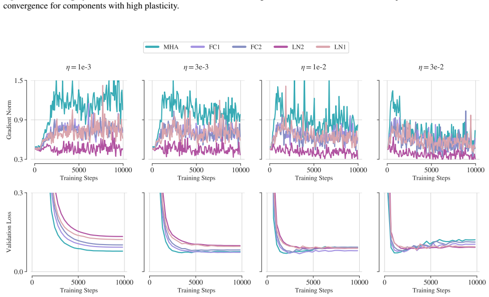
- [Section 5.2, Tables 3 and 6] The cross-group finetuning comparison confounds plasticity with trainable-parameter count. MHA, FC1, and FC2 each update 28M parameters (33% of ViT-Base), while LN1 and LN2 update only 18K (0.02%). The shared four-point learning-rate sweep (Table 5) does not control for capacity; even with optimal learning rates, the expressivity difference could explain the average accuracy gap (90.8% vs. 89.9% in Table 6). The within-group comparisons (MHA>FC1>FC2 and LN2>LN1) are valid evidence because parameter count is fixed within each group, but the cross-group claim in Takeaway 3 requires either matching parameter budgets across groups (e.g., updating multiple LayerNorm layers to reach a comparable parameter count) or using a parameter-efficient adapter on the low-plasticity components.
- [Section 5.2, Fig. 4 (middle)] The gradient-norm comparison is also confounded by parameter count. The norm of the gradient with respect to all trainable parameters of a module typically scales with the number of parameters, so the observation that MHA, FC1, and FC2 have larger gradient norms than LN1 and LN2 may reflect module size rather than plasticity. Reporting per-parameter gradient norms, or the gradient of the output with respect to a fixed-size parameter subset, would separate the two explanations and strengthen the proposed mechanism.
minor comments (5)
- [Section 2, Background] The definition of Lipschitz continuity says 'there exists a constant K≤0'; this should be K≥0, since the Lipschitz constant is nonnegative.
- [Abstract vs. Section 5.2] The abstract states 'over 1,000 finetuning runs,' but Section 5.2 reports 'a total of ∼800 finetuning runs.' Please reconcile these numbers.
- [Proposition 4 proof] In Appendix B.4, the line '∥E∥2∥2vec(pi)∥2' appears to contain a typo; it should be ∥E∥2 ∥vec(pi)∥. Please check all equations in the proof for similar notational slips.
- [Section 3, Terminology] The term 'non-smooth' is used for modules with P(f)>1, but the paper does not claim these modules are non-differentiable. To avoid confusion, state explicitly that 'non-smooth' here means 'high average rate of change,' not lack of differentiability.
- [Figure 2] The left panel's x-axis label 'Theoretical Plasticity Rank' and the middle panel's 'Plasticity Rank' are easy to confuse. Please clarify in the caption which is the theoretical ordering and which is the empirical ordering.
Circularity Check
No significant circularity: the plasticity measure and finetuning outcomes are empirically independent, and the theoretical bounds are not fitted to the target claim.
full rationale
The paper's central derivation is not circular. Plasticity (Definition 1) is an independent, parameter-free measure of average rate of change computed from pretrained weights, with no parameter fitted to finetuning accuracy. The theoretical upper bounds (Propositions 1–4) are standard Lipschitz-type bounds built on external results (e.g., Castin et al., 2024; Nair, 2026) and are not constructed from the finetuning outcomes. The empirical plasticity ranking is measured before finetuning, and the finetuning comparison is a separate optimization procedure. The only self-citations (Odonnat et al., 2025a,b; Xie et al., 2024, 2025; Zekri et al., 2025; Ilbert et al., 2024; Houliston et al., 2025) appear in related work or peripheral remarks and are not load-bearing for the main claim. The difference in trainable parameter count between MHA/FC (28M) and LN (18K) configurations is a real threat to the causal interpretation of the finetuning results, but that is an experimental confound, not a circular reduction of the prediction to its inputs. The theoretical ranking is based on upper bounds, not exact identities, and the empirical validation on the same pretrained model is a consistency check rather than an out-of-sample prediction; neither constitutes circularity under the required standard.
Axiom & Free-Parameter Ledger
free parameters (1)
- token radius bound r =
19.4
axioms (6)
- standard math Matrix norm submultiplicativity inequalities (Lemma 1)
- domain assumption Castin et al. Theorem 3.3: self-attention is Lipschitz on bounded token sequences
- standard math Nair Theorem 1: softmax is 1/2-Lipschitz in l2
- domain assumption All tokens at each position share the same mean and positive standard deviation (Proposition 1)
- domain assumption Images have bounded total energy E and token Frobenius norm is bounded by alpha*sqrt(E)
- ad hoc to paper Weight norms allow comparing upper bounds: gamma entries comparable to W entries; spectral norms above 1
Cite this review
Pith. "Pith review of Vision Transformer Finetuning Benefits from Non-Smooth Components." pith.science (2026). https://pith.science/paper/C43B7LBA
@misc{pith2026260206883,
  author       = {Pith},
  title        = {Pith review of: Vision Transformer Finetuning Benefits from Non-Smooth Components},
  year         = {2026},
  howpublished = {\url{https://pith.science/paper/C43B7LBA}},
  note         = {Machine review of arXiv:2602.06883}
}
read the original abstract
The smoothness of the transformer architecture has been extensively studied in the context of generalization, training stability, and adversarial robustness. However, its role in transfer learning remains poorly understood. In this paper, we analyze the ability of vision transformer components to adapt their outputs to changes in inputs, or, in other words, their \emph{plasticity}. Defined as an average rate of change, it captures the sensitivity to input perturbation; in particular, a high plasticity implies a low smoothness. Our theoretical analysis and extensive experiments -- over $1,000$ finetuning runs on large-scale vision transformers -- showcase that this perspective provides principled guidance in choosing the components to prioritize during adaptation. A key takeaway for practitioners is that the high plasticity of the attention modules and feedforward layers consistently leads to better finetuning performance. Our findings depart from the prevailing assumption that smoothness is desirable, offering a novel perspective on transformers' functional properties. The code is available at https://github.com/ambroiseodt/vit-plasticity.
Figures




Reference graph
Works this paper leans on
-
[6]
URL https: //doi.org/10.1007/978-3-031-20053-3 _29
doi: 10 .1007/978-3-031-20053-3 _29. URL https: //doi.org/10.1007/978-3-031-20053-3 _29. Touvron, H., Lavril, T., Izacard, G., Martinet, X., Lachaux, M.-A., Lacroix, T., Rozière, B., Goyal, N., Hambro, E., Azhar, F., Rodriguez, A., Joulin, A., Grave, E., and Lample, G. Llama: Open and efficient foundation lan- guage models, 2023. URL https://arxiv.org/abs...
Pith/arXiv arXiv 2023
-
[8]
URL https://proceedings.mlr.press/v97/ houlsby19a.html. Hu, E. J., yelong shen, Wallis, P., Allen-Zhu, Z., Li, Y ., Wang, S., Wang, L., and Chen, W. LoRA: Low-rank adaptation of large language models. InInternational Conference on Learning Representations, 2022. URL https://openreview.net/forum?id=nZeVKeeFYf9. HuggingFace. Transformers. https://github.com...
arXiv 2022
-
[10]
URL https://www.cs.toronto.edu/~kriz/ learning-features-2009-TR.pdf. Krogh, A. and Hertz, J. A simple weight decay can improve generalization. In Moody, J., Hanson, S., and Lippmann, R. (eds.),Advances in Neural Information Processing Sys- tems, volume 4. Morgan-Kaufmann, 1991. URL https: //proceedings.neurips.cc/paper_files/paper/ 1991/file/8eefcfdf5990e...
Pith/arXiv arXiv 2009
-
[11]
Curran Associates Inc. ISBN 9781713829546. Li, X. L. and Liang, P. Prefix-tuning: Optimizing con- tinuous prompts for generation. In Zong, C., Xia, F., Li, W., and Navigli, R. (eds.),Proceedings of the 59th Annual Meeting of the Association for Computational Linguistics and the 11th International Joint Conference on Natural Language Processing (Volume 1: ...
Pith/arXiv arXiv 2021
-
[13]
URL https://proceedings.mlr.press/v137/ rosca20a.html. Sander, M. E., Ablin, P., Blondel, M., and Peyré, G. Sink- formers: Transformers with doubly stochastic atten- tion. In Camps-Valls, G., Ruiz, F. J. R., and Valera, I. (eds.),Proceedings of The 25th International Con- ference on Artificial Intelligence and Statistics, volume 151 ofProceedings of Machi...
arXiv 2022
-
[15]
Wang, D., Shelhamer, E., Liu, S., Olshausen, B., and Dar- rell, T
URL https://proceedings.mlr.press/v202/ von-oswald23a.html. Wang, D., Shelhamer, E., Liu, S., Olshausen, B., and Dar- rell, T. Tent: Fully test-time adaptation by entropy mini- mization. InInternational Conference on Learning Rep- resentations, 2021. URL https://openreview.net/ forum?id=uXl3bZLkr3c. Weng, T.-W., Zhang, H., Chen, P.-Y ., Yi, J., Su, D., Ga...
Pith/arXiv arXiv 2021
-
[16]
Zhang, D., Feng, T., Xue, L., Wang, Y ., and Tang, J
URL https://proceedings.mlr.press/v202/ zhai23a.html. Zhang, D., Feng, T., Xue, L., Wang, Y ., and Tang, J. Parameter-efficient fine-tuning for foundation models. arXiv preprint arXiv:2501.13787, 2025. Zhao, B., Tu, H., Wei, C., Mei, J., and Xie, C. Tun- ing layernorm in attention: Towards efficient multi- modal LLM finetuning. InThe Twelfth International...
Pith/arXiv arXiv 2025
-
[17]
Hybrid Architecture
that combines Muon with QK-Norm. Lipschitz constant estimation.A lot of effort has been put into estimating the Lipschitz constants of neural networks. While linear and activation layers have a known tight Lipschitz constant (Béthune et al., 2024; Castin et al., 2024; Virmaux & Scaman, 2018), estimating the Lipschitz constant of feedforward networks is NP...
2024
-
[2005]
Gu, Y ., Han, X., Liu, Z., and Huang, M
ISBN 978-0974707723. Gu, Y ., Han, X., Liu, Z., and Huang, M. PPT: Pre- trained prompt tuning for few-shot learning. In Mure- san, S., Nakov, P., and Villavicencio, A. (eds.),Proceed- ings of the 60th Annual Meeting of the Association for Computational Linguistics (Volume 1: Long Papers), pp. 8410–8423, Dublin, Ireland, May 2022. Associa- tion for Computa...
2022
-
[2009]
CVPR 2009. IEEE Conference on, pp. 248–255. IEEE, 2009. URL https://ieeexplore.ieee.org/ abstract/document/5206848/. Deng, W., Suh, Y ., Gould, S., and Zheng, L. Confidence and dispersity speak: Characterizing prediction matrix for un- supervised accuracy estimation. In Krause, A., Brunskill, E., Cho, K., Engelhardt, B., Sabato, S., and Scarlett, J. (eds....
arXiv 2009
-
[2012]
Houliston, S., Odonnat, A., Arnal, C., and Cabannes, V
ISBN 978-0521548236. Houliston, S., Odonnat, A., Arnal, C., and Cabannes, V . Provable benefits of in-tool learning for large language models, 2025. Houlsby, N., Giurgiu, A., Jastrzebski, S., Morrone, B., De Laroussilhe, Q., Gesmundo, A., Attariyan, M., and Gelly, S. Parameter-efficient transfer learning for NLP. In Chaudhuri, K. and Salakhutdinov, R. (ed...
2025
-
[2016]
URLhttps://arxiv.org/abs/1607.06450. Bartlett, P. For valid generalization the size of the weights is more important than the size of the net- work. In Mozer, M., Jordan, M., and Petsche, T. (eds.),Advances in Neural Information Processing Systems, volume 9. MIT Press, 1996. URL https: //proceedings.neurips.cc/paper_files/paper/ 1996/file/fb2fcd534b0ff3bb...
Pith/arXiv arXiv 1996
-
[2019]
Han, Z., Gao, C., Liu, J., Zhang, J., and Zhang, S
doi: 10.1109/CVPR.2019.00494. Han, Z., Gao, C., Liu, J., Zhang, J., and Zhang, S. Q. Parameter-efficient fine-tuning for large models: A com- prehensive survey.Transactions on Machine Learn- ing Research, 2024. ISSN 2835-8856. URL https: //openreview.net/forum?id=lIsCS8b6zj. Hanson, S. and Pratt, L. Comparing biases for minimal net- work construction with...
arXiv 2019
-
[2020]
Kim, H., Papamakarios, G., and Mnih, A
URLhttps://arxiv.org/abs/2001.08361. Kim, H., Papamakarios, G., and Mnih, A. The lipschitz constant of self-attention. In Meila, M. and Zhang, T. (eds.),Proceedings of the 38th International Conference on Machine Learning, volume 139 ofProceedings of Machine Learning Research, pp. 5562–5571. PMLR, 18– 24 Jul 2021. URL https://proceedings.mlr.press/ v139/k...
Pith/arXiv arXiv 2001
-
[2021]
Dehghani, M., Djolonga, J., Mustafa, B., Padlewski, P., Heek, J., Gilmer, J., Steiner, A
URL https://proceedings.mlr.press/v139/ dasoulas21a.html. Dehghani, M., Djolonga, J., Mustafa, B., Padlewski, P., Heek, J., Gilmer, J., Steiner, A. P., Caron, M., Geirhos, R., Alabdulmohsin, I., Jenatton, R., Beyer, L., Tschan- nen, M., Arnab, A., Wang, X., Riquelme Ruiz, C., Min- derer, M., Puigcerver, J., Evci, U., Kumar, M., Steenkiste, S. V ., Elsayed...
2023
-
[2023]
I Can’t Believe It’s Not Better!
URL https://www.ncbi.nlm.nih.gov/books/ NBK557811/. Updated May 1, 2023. Qu, C., Dai, S., Wei, X., Cai, H., Wang, S., Yin, D., Xu, J., and Wen, J.-R. Tool learning with large language models: A survey.Frontiers of Computer Science, 19(8):198343, 2025. Quionero-Candela, J., Sugiyama, M., Schwaighofer, A., and Lawrence, N. D.Dataset Shift in Machine Learnin...
2023
-
[2025]
Guo, Y ., Shi, H., Kumar, A., Grauman, K., Rosing, T., and Feris, R
URLhttps://arxiv.org/abs/2501.12948. Guo, Y ., Shi, H., Kumar, A., Grauman, K., Rosing, T., and Feris, R. Spottune: Transfer learning through adaptive fine-tuning. In2019 IEEE/CVF Conference on Computer Vision and Pattern Recognition (CVPR), pp. 4800–4809,
discussion (0)
Sign in with ORCID, Apple, or X to comment. Anyone can read and Pith papers without signing in.