REVIEW 4 major objections 6 minor 55 references
This paper claims that fitting k-space measurements in an easy-to-hard order—low frequencies first—lets fully unsupervised deep generative models reconstruct undersampled MRI more accurately and in fewer iterations than uniform fitting.
Reviewed by Pith at T0; open to challenge. T0 means a machine referee read the full paper against a public rubric. the ladder, T0–T4 →
T0 review · deepseek-v4-flash
2026-08-02 22:01 UTC pith:6K7Z7ZTU
load-bearing objection Real empirical recipe and a broken convergence proof; the scheduling idea may be worth stealing, but Theorem VI.1 should not be cited. the 4 major comments →
CogGen: Cognitive-Load-Inspired Fully Unsupervised Deep Generative Modeling for Compressively Sampled MRI Reconstruction
The pith
A machine-rendered reading of the paper's core claim, the machinery that carries it, and where it could break.
Core claim
The central claim is that replacing uniform data-consistency fitting with a cognitive-load-inspired curriculum—where the model first masters low-frequency k-space samples and only later encounters high-frequency and noise-dominated ones—improves both the convergence rate and the final fidelity of fully unsupervised generative reconstruction. Theoretically, the paper shows that when early stages favor easy measurements, the weighted objective has a larger Polyak-Łojasiewicz curvature and lower noise amplification per iteration, yielding a smaller sufficient-iteration bound and a smaller cumulative noise-amplification bound than uniform fitting. If this is right, training-free deep generators
What carries the argument
The central mechanism is the SPCL-driven dual-threshold weighting (CogGen), which assigns each k-space sample a weight v_i = s_i * t_i. The student-mode term s_i includes a sample when its normalized data-consistency residual is below a threshold λ (the model can already fit it), and the teacher-mode term t_i includes samples whose k-space radius is below a growing radius threshold r (physics-informed difficulty). Together these define an easy-to-hard schedule, and the resulting weighted objective is L(θ) = || v⊙(A f_θ(z) − y) ||^2 / || v⊙y ||^2 − λ||v||_1, optimized with alternating updates of v, λ, r, and θ. The proofs then rest on showing that this schedule raises the PL curvature and low
Load-bearing premise
The load-bearing premise is that early curriculum stages make the optimization landscape more strongly curved (a larger Polyak-Łojasiewicz constant) than uniform fitting; the appendix asserts this as an assumption, and for the simplified objective it analyzes, masking alone cannot increase the minimum curvature, so the proof's acceleration conclusion depends on this unproved premise.
What would settle it
Numerically compute the smallest eigenvalue of the weighted data-fidelity Hessian (or the PL constant of the NTK-linearized objective) at the first curriculum stage for a real variable-density mask, both with and without the normalization of Eq. (4), and compare it to the uniform case. If the early-stage curvature is not strictly larger, Theorem VI.1's premise fails and the accelerated-convergence argument collapses.
If this is right
- Fully unsupervised MRI reconstruction can beat supervised models on the reported benchmark slices without any paired training data.
- A fixed iteration budget goes further: early curricula roughly halve the convergence time needed to reach a given fidelity.
- Both architectural families (DIP and INR) benefit, meaning the scheduling insight can be ported to other untrained generators.
- The approach gives a principled explanation for why 'easy first' training helps in inverse problems: it avoids feeding the model noise-dominated directions early.
- If the noise-amplification theory holds, CogGen-like schedules should degrade gracefully as measurement noise increases.
Where Pith is reading between the lines
- The cognitive-load framing is a metaphor; the actual content is a weighted least-squares continuation method, so similar gains might appear in other ill-posed linear inverse problems whose measurements have a frequency or scale structure.
- A testable extension is to replace the fixed radius and residual thresholds with a learned or submodular selection of k-space points, which the authors flag as future work and which could tighten the practical gains.
- Because the proof relies on the PL constant being larger for the weighted objective, one could try to construct masks that provably increase a measure of effective curvature—if that is impossible, the gains must instead come from the normalization term the analysis does not treat.
- The reported gains are on single-slice retrospective data; an unexplored consequence is whether the curriculum also helps multi-coil or dynamic MRI, where the measurement structure is richer.
Editorial analysis
A structured set of objections, weighed in public.
Referee Report
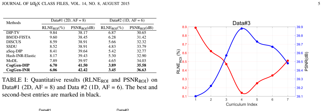
Summary. The paper proposes CogGen, an unsupervised CS-MRI reconstruction framework that schedules k-space measurements from low-frequency (easy) to high-frequency (hard) via a self-paced curriculum weighting that combines a residual-based student threshold and a k-space-radius teacher threshold. Two instantiations are built on DIP and INR backbones. The paper reports quantitative gains on two single-slice datasets (Table I) and ablations on a third, and provides appendices purporting to prove that the curriculum lowers the PL-based iteration bound (Theorem VI.1) and reduces cumulative noise amplification (Appendix B). The central theoretical claim is that early weighting enlarges the PL constant; the empirical claim is that CogGen outperforms supervised and unsupervised baselines.
Significance. If the empirical gains are reproducible, the k-space curriculum idea is a simple and practical contribution to unsupervised DIP/INR reconstruction. Table I shows large PSNR/RLNE differences, and the ablations (Figs. 4-6) are internally consistent and support the value of the dual-mode weighting. However, the advertised theoretical support is not valid as written: Theorem VI.1 rests on an assumption contradicted by the Hessian calculation in the same appendix, and Appendix B's bound is built into the noise-energy assumption. The empirical evaluation is also too thin (single slices, no error bars) to establish the headline claim, and the authors' own Future Work acknowledges the weighting rule is semi-empirical. With corrected theory and broader evaluation, the contribution could be valuable.
major comments (4)
- [Appendix A, Eq. (A.9) / Theorem VI.1] The premise μ_t ≥ μ_early > μ_uniform in (A.9) is inconsistent with the Hessian in (A.4). For V^(t)=diag(v_i) with v_i∈[0,1] (w1,w2∈(0.5,1]), V²⪯I, so A^H V² A ⪯ A^H A and hence λ_min(H_t) ≤ λ_min(H_uniform) for the same Jacobian J_t. Row-weighting cannot enlarge the PL constant of the unnormalized objective (A.1); it can only reduce it. The bound k_CogGen < k_DIP therefore follows directly from an assumption that contradicts the model analyzed. If the intended mechanism is the normalization by ||v⊙y||² in Eq. (4)/(6), that normalization is never analyzed. This is a load-bearing gap for the advertised convergence guarantee.
- [Appendix B, Eq. (A.11)] The inequality B_CogGen < B_DIP is hard-wired through the assumption that ||v^(t)_CogGen ε|| ≤ bar_v ||ε|| with bar_v<1 for early t. That assumption, not any property of the proposed scheduling, produces the improvement. The proof also never ties v^(t) to the dual-threshold rule (Eq. 5) or to the normalized loss actually minimized (Eq. 6). The result says only that if early stages suppress some noise energy, the cumulative noise bound is smaller; it does not establish a property of CogGen. Please either analyze the true update or label this as a heuristic motivation rather than a proof.
- [Section IV-A, Table I, Figs. 2-3] The headline empirical claim is based on one retrospectively downsampled slice per dataset for Data#1 and Data#2, and Data#3 is used only for ablations. No error bars, multiple runs, or statistical tests are reported. Table I shows large PSNR/RLNE differences, but with n=1 per condition the claim of superiority over supervised methods (MoDL) and self-supervised methods (SSDU) is not statistically supported. Please report results over multiple slices/subjects with variance and a paired test.
- [Eq. (4) vs Algorithm 1] Eq. (4) presents a joint optimization over θ and v with regularizer −λ||v||_1, but Algorithm 1 never minimizes over v; v is assigned by the threshold rules in Eq. (5). The relationship between the SPCL objective and the implemented schedule should be clarified. As written, the appendix analyzes a different loss from the one minimized in Algorithm 1.
minor comments (6)
- [Sec. II-B] The steady-state expression e_i^{(∞)} ≈ ε_i/σ_i divides by σ_i; for σ_i=0 (unmeasured k-space directions) it is undefined. State that the recursion is restricted to positive singular values or use the pseudoinverse.
- [Eq. (A.1)/(A.4)] v^(t) is used both as a vector and as a diagonal operator V^(t); distinguish the two notations.
- [Lemma VI.1] L_t is used for both the objective and the Lipschitz constant; use different symbols to avoid confusion in the step-size condition η≤1/L_t.
- [Table I/Table II] Table I's caption says entries are 'marked in black', but no bold/color is visible; Table II has inconsistent spacing (CogGen CL -INR).
- [Algorithm 1] Line 4 uses K_2(k_1) without definition; the later values K_2=[1000,1000,2000,2000,10000] should be stated in the algorithm.
- [Appendix B] The first noise bound has an undefined constant α that later disappears, and the text cross-references 'VI-B' instead of an equation number.
Circularity Check
Theorem VI.1's faster-convergence claim is assumption (A.9) restated: k_CogGen < k_DIP is exactly μ_early > μ_uniform, and the proof invokes (A.9) directly.
specific steps
-
self definitional
[Appendix A, Eqs. (A.9)-(A.10) and proof of Theorem VI.1]
"Assume that CogGen constructs a curriculum {v^(t)} such that, during an early phase t≤t0, μ_t ≥ μ_early > μ_uniform. (A.9) ... Requiring the right-hand side to be no larger than ρ yields k ≥ log(1/ρ)/(η μ_t). Using (A.9) completes the proof."
Lemma VI.1 gives the iteration count k = log(1/ρ)/(η μ_t), so Theorem VI.1's inequality k_CogGen < k_DIP is exactly the assumed inequality μ_early > μ_uniform. The proof adds nothing beyond 'Using (A.9) completes the proof': the predicted acceleration is the premise restated. Moreover, for the unnormalized objective (A.1) the Hessian is H_t = 2 J^H A^H (V^(t))^2 A J (A.4); since V² ⪯ I, H_t ⪯ H_uniform and λ_min(H_t) ≤ λ_min(H_uniform), so μ_t ≤ μ_uniform, contradicting (A.9). The heuristic that masking 'removes near-null directions' is backwards: downweighting rows of A enlarges the nullspace. Hence the advertised bound is not derived from CogGen's update.
full rationale
The empirical part of the paper is self-contained: CogGen-DIP and CogGen-INR are compared against external baselines on three in-vivo datasets, and the ablations are genuine experiments. That portion is not circular. The circularity is confined to the advertised convergence theory. In Appendix A, μ_t is defined as the PL constant of the weighted objective, and Lemma VI.1 immediately yields convergence at rate 1/μ_t. Theorem VI.1 then 'proves' k_CogGen < k_DIP by assuming μ_early > μ_uniform in (A.9); the proof itself says 'Using (A.9) completes the proof.' Thus the central theoretical prediction is an assumption restated, not a consequence of the scheduling rule. In addition, the assumption is inconsistent with the objective actually analyzed: with V^(t) diagonal entries ≤1, the weighted Hessian is PSD-dominated by the uniform Hessian, so the minimum PL curvature can only decrease, not increase. The normalized objective in Eq. (4) could in principle supply the needed conditioning improvement, but the appendix does not analyze that normalization. The noise-imprint bound in Appendix B is a straightforward consequence of its explicit assumption \bar v < 1 and is not counted as a separate circular step. No load-bearing self-citation was found. Overall: one central 'prediction' reduces by construction, so score 6.
Axiom & Free-Parameter Ledger
free parameters (4)
- residual threshold schedule (lambda, Delta lambda) =
not specified; 'initial values ... from small magnitudes' and exponential growth
- radius threshold schedule (r, Delta r) =
not specified
- weighting factors w1, w2 =
only ranges w1, w2 in (0.5,1] given
- curriculum length K1 and per-stage iteration budget K2 =
K1=5; K2=[1000,1000,2000,2000,10000] on Data#1/2; stage count tuned on Data#3
axioms (5)
- domain assumption Observation noise is additive white Gaussian and the forward model is y = Ax + eps (Eq. 1)
- domain assumption NTK-style local linearization f_theta(z) ≈ f_{theta_t}(z) + J_t(theta - theta_t) (Eq. A.2)
- domain assumption Weighted objective satisfies PL inequality with mu_t > 0 (Eq. A.6)
- ad hoc to paper Early-stage PL constant satisfies mu_t >= mu_early > mu_uniform (Eq. A.9)
- standard math Weighted updates are non-expansive: ||I - eta A^* v A|| <= rho_t < 1 (Appendix B)
read the original abstract
Fully unsupervised deep generative modeling (FU-DGM) offers significant potential for compressively sampled magnetic resonance imaging (CS-MRI) reconstruction. Representative FU-DGM formulations, such as deep image prior (DIP) and implicit neural representation (INR), employ architectural bias to induce a low-dimensional manifold in the image space that aligns with the forward observation. However, as the underlying inverse system is highly ill-posed, prolonged iterative fitting in FU-DGM typically leads to poor efficiency and noise amplification. In this paper, guided by the cognitive principle of easy-to-hard learning, we propose CogGen, an FU-DGM framework that reformulates CS-MRI reconstruction as a staged inversion problem. Specifically, CogGen implements an self-paced curriculum learning (SPCL)-driven progressive scheduling strategy through an MRI-aware dual-threshold weighting criterion, which adaptively regulates k-space measurement participation. The data-consistency residual thresholding evaluates the fitting reliability of the current generator, while the k-space radius thresholding controls stage-wise measurement exposure, thereby avoiding uniform fitting throughout optimization. Theoretically, our analysis shows that, when early stages favor easy-to-fit measurements, CogGen yields a reduced local sufficient-iteration bound and a smaller cumulative noise-amplification bound, explaining the improved convergence behavior and reconstruction fidelity of CogGen within a finite iteration budget. Numerical experiments demonstrate that both CogGen instantiations, CogGen-DIP and CogGen-INR, achieve superior performance over prevailing CS-MRI reconstruction techniques, including unsupervised and supervised pipelines.
Figures




Reference graph
Works this paper leans on
-
[1]
Modern diagnostic imaging technique applications and risk factors in the medical field: a review,
S. Hussain, I. Mubeen, N. Ullah, S. S. U. D. Shah, B. A. Khan, M. Zahoor, R. Ullah, F. A. Khan, and M. A. Sultan, “Modern diagnostic imaging technique applications and risk factors in the medical field: a review,”BioMed research international, vol. 2022, no. 1, p. 5164970, 2022
2022
-
[2]
Next-generation mri scanner designed for ultra- high-resolution human brain imaging at 7 tesla,
D. A. Feinberg, A. J. Beckett, A. T. Vu, J. Stockmann, L. Huber, S. Ma, S. Ahn, K. Setsompop, X. Cao, S. Park JOURNAL OF LATEX CLASS FILES, VOL. 14, NO. 8, AUGUST 2015 8 et al., “Next-generation mri scanner designed for ultra- high-resolution human brain imaging at 7 tesla,”Nature methods, vol. 20, no. 12, pp. 2048–2057, 2023
2015
-
[3]
2.5-minute fast brain mri with multiple contrasts in acute ischemic stroke,
A. Kits, J. Al-Saadi, F. De Luca, F. Janzon, M. V. Mazya, J. Lundberg, T. Sprenger, S. Skare, and A. F. Delgado, “2.5-minute fast brain mri with multiple contrasts in acute ischemic stroke,”Neuroradiology, vol. 66, no. 5, pp. 737– 747, 2024
2024
-
[4]
Emerging techniques in cardiac magnetic resonance imaging,
R. Guo, S. Weing ¨artner, P. ˇSiuryt˙e, C. T Stoeck, M. F¨ uetterer, A. E Campbell-Washburn, A. Suinesiaputra, M. Jerosch-Herold, and R. Nezafat, “Emerging techniques in cardiac magnetic resonance imaging,”Journal of Mag- netic Resonance Imaging, vol. 55, no. 4, pp. 1043–1059, 2022
2022
-
[5]
Compressed sensing: From research to clinical practice with deep neural networks: Shortening scan times for magnetic resonance imaging,
C. M. Sandino, J. Y. Cheng, F. Chen, M. Mardani, J. M. Pauly, and S. S. Vasanawala, “Compressed sensing: From research to clinical practice with deep neural networks: Shortening scan times for magnetic resonance imaging,” IEEE signal processing magazine, vol. 37, no. 1, pp. 117– 127, 2020
2020
-
[6]
Recent advances in parallel imaging for mri: Wave-caipi technique,
C. Curatolo, “Recent advances in parallel imaging for mri: Wave-caipi technique,”Journal of Advanced Health Care, vol. 4, no. 1, 2022
2022
-
[7]
A review on accel- erated magnetic resonance imaging techniques: Parallel imaging, compressed sensing, and machine learning,
M. Tavakkoli and M. Noseworthy, “A review on accel- erated magnetic resonance imaging techniques: Parallel imaging, compressed sensing, and machine learning,” Critical Reviews™in Biomedical Engineering, 2025
2025
-
[8]
An introduction to deep generative modeling,
L. Ruthotto and E. Haber, “An introduction to deep generative modeling,”GAMM-Mitteilungen, vol. 44, no. 2, p. e202100008, 2021
2021
-
[9]
A survey of multimodal deep generative models,
M. Suzuki and Y. Matsuo, “A survey of multimodal deep generative models,”Advanced Robotics, vol. 36, no. 5-6, pp. 261–278, 2022
2022
-
[10]
Mathematical models for magnetic resonance imaging reconstruction: An overview of the approaches, problems, and future research areas,
M. Doneva, “Mathematical models for magnetic resonance imaging reconstruction: An overview of the approaches, problems, and future research areas,” IEEE Signal Process. Mag., vol. 37, no. 1, pp. 24–32, 2020
2020
-
[11]
Dagan: Deep de-aliasing generative adversarial networks for fast compressed sensing mri reconstruction,
G. Yang, S. Yu, H. Dong, G. Slabaugh, P. L. Dragotti, X. Ye, F. Liu, S. Arridge, J. Keegan, Y. Guo, and D. Firmin, “Dagan: Deep de-aliasing generative adversarial networks for fast compressed sensing mri reconstruction,”IEEE Transactions on Medical Imaging, vol. 37, no. 6, pp. 1310–1321, 2018
2018
-
[12]
Com- pressed sensing mri reconstruction using a generative adversarial network with a cyclic loss,
T. M. Quan, T. Nguyen-Duc, and W.-K. Jeong, “Com- pressed sensing mri reconstruction using a generative adversarial network with a cyclic loss,”IEEE Transactions on Medical Imaging, vol. 37, no. 6, pp. 1488–1497, 2018
2018
-
[13]
High quality and fast compressed sensing mri reconstruction via edge-enhanced dual discriminator generative adversarial network,
Y. Li, J. Li, F. Ma, S. Du, and Y. Liu, “High quality and fast compressed sensing mri reconstruction via edge-enhanced dual discriminator generative adversarial network,”Mag- netic Resonance Imaging, vol. 77, pp. 124–136, 2021
2021
-
[14]
Unpaired deep learning for accelerated mri using optimal transport driven cyclegan,
G. Oh, B. Sim, H. Chung, L. Sunwoo, and J. C. Ye, “Unpaired deep learning for accelerated mri using optimal transport driven cyclegan,”IEEE Transactions on Com- putational Imaging, vol. 6, pp. 1285–1296, 2020
2020
-
[15]
Learning mri artefact removal with unpaired data,
S. Liu, K.-H. Thung, L. Qu, W. Lin, D. Shen, and P.-T. Yap, “Learning mri artefact removal with unpaired data,” Nature Machine Intelligence, vol. 3, no. 1, pp. 60–67, 2021
2021
-
[16]
Time-dependent deep image prior for dynamic mri,
J. Yoo, K. H. Jin, H. Gupta, J. Yerly, M. Stuber, and M. Unser, “Time-dependent deep image prior for dynamic mri,”IEEE Transactions on Medical Imaging, vol. 40, no. 12, pp. 3337–3348, 2021
2021
-
[17]
Accelerated mri with un-trained neural networks,
M. Z. Darestani and R. Heckel, “Accelerated mri with un-trained neural networks,”IEEE Transactions on Com- putational Imaging, vol. 7, pp. 724–733, 2021
2021
-
[18]
Nerp: implicit neural representation learning with prior embedding for sparsely sampled image reconstruction,
L. Shen, J. Pauly, and L. Xing, “Nerp: implicit neural representation learning with prior embedding for sparsely sampled image reconstruction,”IEEE Transactions on Neural Networks and Learning Systems, vol. 35, no. 1, pp. 770–782, 2022
2022
-
[19]
Pearl: Cascaded self-supervised cross-fusion learning for parallel mri acceleration,
Q. Zhu, B. Liu, Z.-X. Cui, C. Cao, X. Yan, Y. Liu, J. Cheng, Y. Zhou, Y. Zhu, H. Wang, H. Zeng, and D. Liang, “Pearl: Cascaded self-supervised cross-fusion learning for parallel mri acceleration,”IEEE Journal of Biomedical and Health Informatics, vol. 29, no. 5, pp. 3086–3097, 2025
2025
-
[20]
Analysis of deep image prior and exploiting self-guidance for image reconstruction,
S. Liang, E. Bell, Q. Qu, R. Wang, and S. Ravishankar, “Analysis of deep image prior and exploiting self-guidance for image reconstruction,”IEEE Transactions on Compu- tational Imaging, 2025
2025
-
[22]
The development of cognitive load theory: Replication crises and incorporation of other theories can lead to theory expansion,
J. Sweller, “The development of cognitive load theory: Replication crises and incorporation of other theories can lead to theory expansion,”Educational Psychology Review, vol. 35, no. 4, p. 95, 2023
2023
-
[23]
A cognitive load theory approach to defining and measuring task complexity through element interactivity,
O. Chen, F. Paas, and J. Sweller, “A cognitive load theory approach to defining and measuring task complexity through element interactivity,”Educational Psychology Review, vol. 35, no. 2, p. 63, 2023
2023
-
[24]
Self-paced curriculum learning,
L. Jiang, D. Meng, Q. Zhao, S. Shan, and A. Hauptmann, “Self-paced curriculum learning,” inProceedings of the AAAI Conference on Artificial Intelligence, vol. 29, no. 1, 2015
2015
-
[25]
Leveraging prior-knowledge for weakly supervised object detection under a collaborative self-paced curriculum learning framework,
D. Zhang, J. Han, L. Zhao, and D. Meng, “Leveraging prior-knowledge for weakly supervised object detection under a collaborative self-paced curriculum learning framework,”International Journal of Computer Vision, vol. 127, no. 4, pp. 363–380, 2019
2019
-
[26]
Screenernet: Learning self-paced curriculum for deep neural networks,
T.-H. Kim and J. Choi, “Screenernet: Learning self-paced curriculum for deep neural networks,”arXiv preprint arXiv:1801.00904, 2018
Pith/arXiv arXiv 2018
-
[27]
Brain-guided self- paced curriculum learning for adaptive human–machine interfaces,
Y.-W. Choi, H.-B. Shin, and S.-W. Lee, “Brain-guided self- paced curriculum learning for adaptive human–machine interfaces,”IEEE Transactions on Systems, Man, and Cybernetics: Systems, 2025
2025
-
[28]
Phase retrieval using untrained neural network priors,
G. Jagatap and C. Hegde, “Phase retrieval using untrained neural network priors,” inNeurIPS 2019 Workshop on Solving Inverse Problems with Deep Networks, 2019
2019
-
[29]
Deeptensor: Low-rank tensor decomposition with deep network priors,
V. Saragadam, R. Balestriero, A. Veeraraghavan, and R. G. Baraniuk, “Deeptensor: Low-rank tensor decomposition with deep network priors,”IEEE Transactions on Pattern JOURNAL OF LATEX CLASS FILES, VOL. 14, NO. 8, AUGUST 2015 9 Analysis and Machine Intelligence, 2024
2015
-
[30]
Denoising and regular- ization via exploiting the structural bias of convolutional generators,
R. Heckel and M. Soltanolkotabi, “Denoising and regular- ization via exploiting the structural bias of convolutional generators,” 2020
2020
-
[31]
Convergence guarantees of overparametrized wide deep inverse prior,
N. Buskulic, Y. Qu ´eau, and J. Fadili, “Convergence guarantees of overparametrized wide deep inverse prior,” pp. 406–417, 2023
2023
-
[32]
Convergence and recovery guarantees of unsupervised neural networks for inverse problems,
N. Buskulic, J. Fadili, and Y. Qu ´eau, “Convergence and recovery guarantees of unsupervised neural networks for inverse problems,”Journal of Mathematical Imaging and Vision, vol. 66, no. 4, pp. 584–605, 2024
2024
-
[33]
Curriculum learning,
Y. Bengio, J. Louradour, R. Collobert, and J. Weston, “Curriculum learning,” inProceedings of the 26th annual international conference on machine learning, 2009, pp. 41–48
2009
-
[34]
Self-paced learning for latent variable models,
M. Kumar, B. Packer, and D. Koller, “Self-paced learning for latent variable models,” vol. 23, 2010
2010
-
[35]
A theoretical understand- ing of self-paced learning,
D. Meng, Q. Zhao, and L. Jiang, “A theoretical understand- ing of self-paced learning,”Information Sciences, vol. 414, pp. 319–328, 2017
2017
-
[36]
Self-paced learning with diversity,
L. Jiang, D. Meng, S.-I. Yu, Z. Lan, S. Shan, and A. G. Hauptmann, “Self-paced learning with diversity,”Ad- vances in neural information processing systems, vol. 27, 2014
2014
-
[37]
Modl: Model- based deep learning architecture for inverse problems,
H. K. Aggarwal, M. P. Mani, and M. Jacob, “Modl: Model- based deep learning architecture for inverse problems,” IEEE transactions on medical imaging, vol. 38, no. 2, pp. 394–405, 2018
2018
-
[38]
fastmri: A publicly available raw k- space and dicom dataset of knee images for accelerated mr image reconstruction using machine learning,
F. Knoll, J. Zbontar, A. Sriram, M. J. Muckley, M. Bruno, A. Defazio, M. Parente, K. J. Geras, J. Katsnelson, H. Chandaranaet al., “fastmri: A publicly available raw k- space and dicom dataset of knee images for accelerated mr image reconstruction using machine learning,”Radiology: Artificial Intelligence, vol. 2, no. 1, p. e190007, 2020
2020
-
[39]
Incorporating reference in parallel imaging and compressed sensing,
X. Peng, L. Ying, Q. G. Liu, Y. J. Zhu, Y. Y. Liu, X. B. Qu, X. Liu, H. R. Zheng, and D. Liang, “Incorporating reference in parallel imaging and compressed sensing,” Magnetic Resonance in Medicine, vol. 73, no. 4, pp. 1490– 1504, 2015
2015
-
[40]
Image restora- tion using total variation regularized deep image prior,
J. Liu, Y. Sun, X. Xu, and U. S. Kamilov, “Image restora- tion using total variation regularized deep image prior,” inICASSP 2019-2019 IEEE International Conference on Acoustics, Speech and Signal Processing (ICASSP). Ieee, 2019, pp. 7715–7719
2019
-
[41]
Decoupled algorithm for mri reconstruc- tion using nonlocal block matching model: Bm3d-mri,
E. M. Eksioglu, “Decoupled algorithm for mri reconstruc- tion using nonlocal block matching model: Bm3d-mri,” Journal of Mathematical Imaging and Vision, vol. 56, no. 3, pp. 430–440, 2016
2016
-
[42]
An unsupervised method for mri recovery: deep image prior with structured sparsity,
M. A. Sultan, C. Chen, Y. Liu, K. Gil, K. Zareba, and R. Ahmad, “An unsupervised method for mri recovery: deep image prior with structured sparsity,”Magnetic Resonance Materials in Physics, Biology and Medicine, pp. 1–13, 2025
2025
-
[43]
Self-supervised learning of physics-guided reconstruction neural networks without fully sampled reference data,
B. Yaman, S. A. H. Hosseini, S. Moeller, J. Ellermann, K. U ˘gurbil, and M. Akc ¸akaya, “Self-supervised learning of physics-guided reconstruction neural networks without fully sampled reference data,”Magnetic resonance in medicine, vol. 84, no. 6, pp. 3172–3191, 2020
2020
-
[44]
Image reconstruction via autoencoding sequential deep image prior,
I. Alkhouri, S. Liang, E. Bell, Q. Qu, R. Wang, and S. Ravishankar, “Image reconstruction via autoencoding sequential deep image prior,”Advances in Neural Infor- mation Processing Systems, vol. 37, pp. 18 988–19 012, 2024
2024
-
[45]
Spatiotemporal implicit neural representation for unsupervised dynamic mri re- construction,
J. Feng, R. Feng, Q. Wu, X. Shen, L. Chen, X. Li, L. Feng, J. Chen, Z. Zhang, C. Liuet al., “Spatiotemporal implicit neural representation for unsupervised dynamic mri re- construction,”IEEE Transactions on Medical Imaging, 2025
2025
-
[46]
Learning interpretable decision rule sets: A submodular optimization approach,
F. Yang, K. He, L. Yang, H. Du, J. Yang, B. Yang, and L. Sun, “Learning interpretable decision rule sets: A submodular optimization approach,”Advances in Neural Information Processing Systems, vol. 34, pp. 27 890– 27 902, 2021
2021
-
[47]
Data- efficient structured pruning via submodular optimization,
M. El Halabi, S. Srinivas, and S. Lacoste-Julien, “Data- efficient structured pruning via submodular optimization,” Advances in Neural Information Processing Systems, vol. 35, pp. 36 613–36 626, 2022
2022
-
[48]
Greedy guarantees for minimum submodular cost submodular/non-submodular cover problem,
M. Shi, Z. Yang, and W. Wang, “Greedy guarantees for minimum submodular cost submodular/non-submodular cover problem,”Journal of Combinatorial Optimization, vol. 45, no. 1, p. 8, 2023
2023
-
[49]
Weak submodularity implies localizability: Local search for constrained non- submodular function maximization,
M. Shi, Q. Zhu, B. Liu, and Y. Li, “Weak submodularity implies localizability: Local search for constrained non- submodular function maximization,”Discrete Mathemat- ics, vol. 348, no. 2, p. 114287, 2025
2025
-
[50]
Neural tangent kernel: Convergence and generalization in neural net- works,
A. Jacot, F. Gabriel, and C. Hongler, “Neural tangent kernel: Convergence and generalization in neural net- works,”Advances in neural information processing sys- tems, vol. 31, 2018
2018
-
[51]
Neural tangent kernel: A survey,
E. Golikov, E. Pokonechnyy, and V. Korviakov, “Neural tangent kernel: A survey,”arXiv preprint arXiv:2208.13614, 2022
Pith/arXiv arXiv 2022
-
[52]
Neural net- works can learn representations with gradient descent,
A. Damian, J. Lee, and M. Soltanolkotabi, “Neural net- works can learn representations with gradient descent,” inConference on Learning Theory. PMLR, 2022, pp. 5413–5452
2022
-
[53]
Linear convergence of gradient and proximal-gradient methods under the polyak- lojasiewicz condition,
H. Karimi, J. Nutini, and M. Schmidt, “Linear convergence of gradient and proximal-gradient methods under the polyak- lojasiewicz condition,” inJoint European confer- ence on machine learning and knowledge discovery in databases. Springer, 2016, pp. 795–811
2016
-
[54]
A generalized alternat- ing method for bilevel learning under the polyak-{\L} ojasiewicz condition,
Q. Xiao, S. Lu, and T. Chen, “A generalized alternat- ing method for bilevel learning under the polyak-{\L} ojasiewicz condition,”arXiv preprint arXiv:2306.02422, 2023
Pith/arXiv arXiv 2023
-
[55]
A. B. Nejma, “Polyak-{\L}ojasiewicz inequality is es- sentially no more general than strong convexity for𝑐 2 functions,”arXiv preprint arXiv:2512.05285, 2025
arXiv 2025
-
[56]
Range restricted iterative methods for linear discrete ill-posed problems,
A. Buccini, L. Onisk, L. Reichelet al., “Range restricted iterative methods for linear discrete ill-posed problems,” Electronic Transactions on Numerical Analysis, vol. 58, pp. 348–377, 2023
2023
discussion (0)
Sign in with ORCID, Apple, or X to comment. Anyone can read and Pith papers without signing in.