Recognition: unknown
Physics-Informed Neural Networks for Maximizing Quantum Fisher Information in Time-Dependent Many-Body Systems
Pith reviewed 2026-05-10 05:16 UTC · model grok-4.3
The pith
Physics-informed neural networks learn counter-diabatic protocols that maximize quantum Fisher information beyond Euler-Lagrange references in driven many-body systems.
A machine-rendered reading of the paper's core claim, the machinery that carries it, and where it could break.
Core claim
The PINN framework, by variationally learning the counter-diabatic driving term together with the scheduling function while enforcing the Euler-Lagrange condition via a Magnus-expanded time-evolution operator, produces protocols that achieve systematically higher normalized quantum Fisher information, favorable fidelity, and low physical residuals than reference solutions based solely on the Euler-Lagrange condition for families of driven spin Hamiltonians up to six qubits.
What carries the argument
A variational physics-informed neural network loss that incorporates the Magnus expansion of the time-ordered exponential to infer the adiabatic gauge potential and scheduling function while satisfying the Euler-Lagrange structure of the counter-diabatic protocol.
If this is right
- The framework yields high normalized QFI together with favorable fidelity and extremal-balance metrics.
- Small physical residuals are preserved while performance exceeds that of reference Euler-Lagrange solutions.
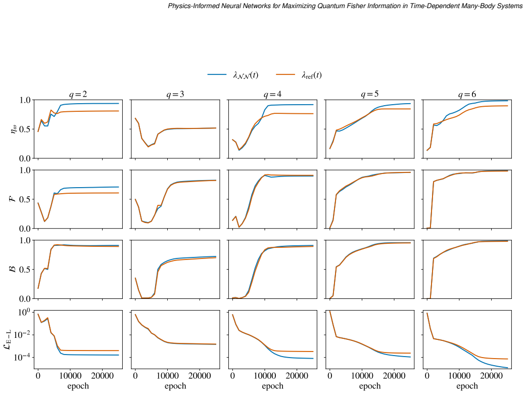
- Explicitly learning the scheduling function provides a performance advantage in most tested cases.
- Non-trivial finite-size effects appear, with the q=3 regime emerging as particularly challenging.
Where Pith is reading between the lines
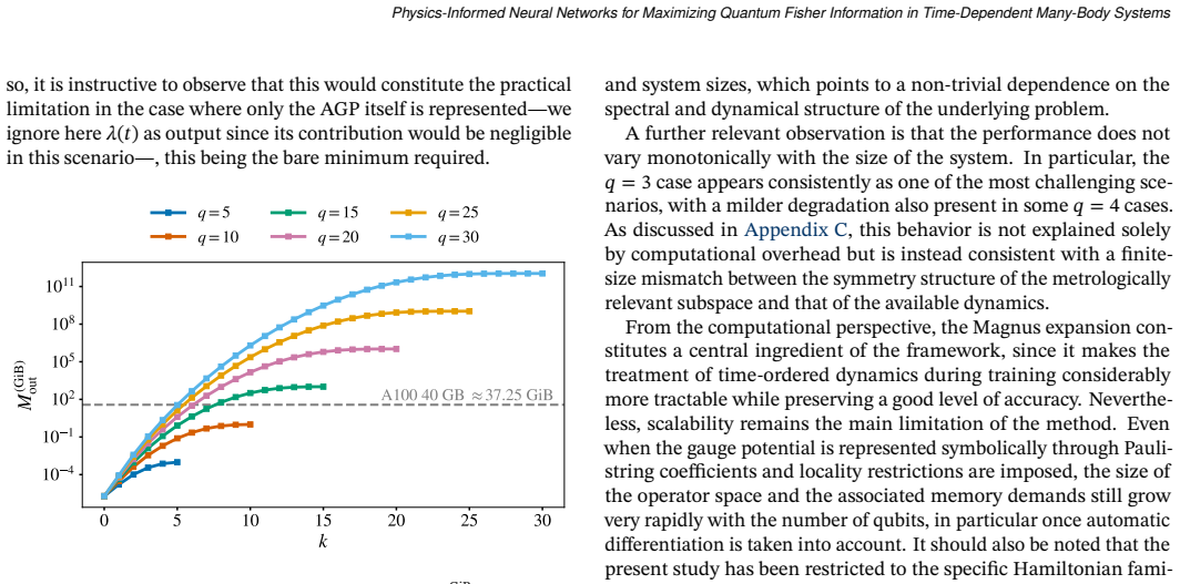
- The exponential growth of the operator space noted in the paper implies that hybrid approximations such as tensor-network representations of the Magnus terms would be needed to reach larger qubit numbers.
- The same variational-PINN structure could be reused for other inverse quantum-control problems that require enforcing adiabatic or counter-diabatic conditions.
- Finite-size effects highlighted for q=3 suggest that the method may reveal scaling laws for metrological advantage in small interacting systems before the large-N limit is taken.
Load-bearing premise
The Magnus-expansion truncation combined with the variational PINN loss accurately captures the true time-ordered dynamics and the learned protocols remain optimal when the Hilbert-space dimension grows beyond six qubits.
What would settle it
Applying the trained networks to a seven-qubit instance of the same Hamiltonians and observing that the achieved normalized QFI falls below the reference Euler-Lagrange value or that the physical residuals become large would falsify the claim of systematic improvement.
Figures


read the original abstract
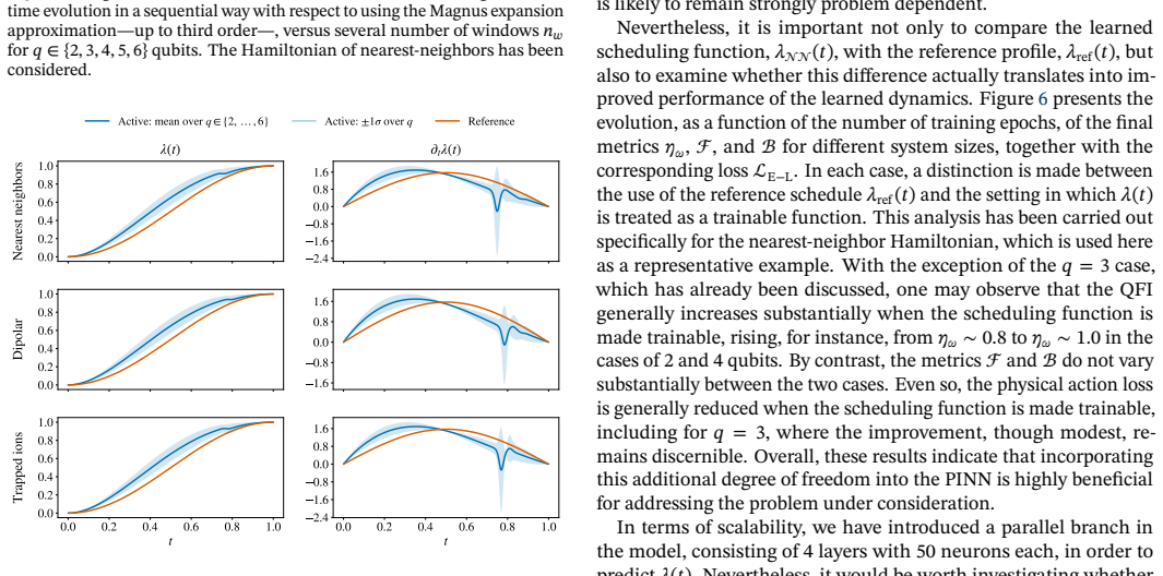
Quantum Fisher Information (QFI) sets the ultimate precision limit for parameter estimation and is therefore a central quantity in quantum metrology. In time-dependent many-body systems, however, maximizing QFI is a highly non-trivial task due to the combined effects of non-commutativity, control complexity, and the exponential growth of the Hilbert space. In this work, we present a physics-informed neural network (PINN) framework to address this problem through the learning of counter-diabatic quantum dynamics. Our approach combines a variational PINN formulation with a Magnus-expansion treatment of time-ordered evolution, enabling the adiabatic gauge potential and the scheduling function to be inferred directly from the underlying physics while enforcing the Euler-Lagrange structure of the protocol. The method is applied to several families of driven spin Hamiltonians, including nearest-neighbor, dipolar, and trapped-ion-inspired interactions, for systems of up to six qubits. The numerical results show that the proposed framework systematically improves over reference solutions based only on the Euler-Lagrange condition, yielding high normalized QFI together with favorable fidelity and extremal-balance metrics while preserving small phsical residuals. The analysis further shows that learning the scheduling function provides a clear performance advantage in most cases, and reveals non-trivial finite-size effects, with $q=3$ emerging as a particularly challenging regime. Although scalability remains limited by the exponential growth of the operator space and by automatic-differentiation costs, the results demonstrate that PINNs constitute a viable and physically grounded route for learning metrologically optimal control strategies in interacting quantum systems.
Editorial analysis
A structured set of objections, weighed in public.
Referee Report
Summary. The paper proposes a physics-informed neural network (PINN) framework that combines a variational formulation with a Magnus-expansion treatment of time-ordered evolution to learn counter-diabatic protocols maximizing the quantum Fisher information (QFI) in time-dependent many-body spin systems. It is applied to nearest-neighbor, dipolar, and trapped-ion-inspired Hamiltonians for up to six qubits, claiming systematic improvements in normalized QFI, fidelity, and extremal-balance metrics over Euler-Lagrange references while keeping small physical residuals, with additional observations on the benefit of learning the scheduling function and finite-size effects (e.g., q=3 regime).
Significance. If the central claims hold after independent verification, the work offers a concrete, physics-constrained numerical route for optimal quantum control in metrology problems on small interacting systems. It explicitly demonstrates the advantage of learning scheduling functions, reports results across multiple Hamiltonian families, and identifies non-trivial finite-size effects, providing a reproducible benchmark set that could guide future extensions of PINNs to quantum sensing protocols.
major comments (3)
- [Abstract and Magnus-expansion treatment] Abstract and Magnus-expansion treatment: the time-evolution operator is obtained from a truncated Magnus series whose truncation order and error relative to the exact time-ordered exponential are neither specified nor validated for the learned controls (up to 6 qubits). Because the variational loss and all reported QFI/fidelity metrics are computed inside this approximation, systematic bias in the Magnus approximant directly affects the optimality assertion and the claimed improvement over references.
- [Abstract] Abstract: the central claim that the PINN 'systematically improves over reference solutions based only on the Euler-Lagrange condition' is circular, since both the network loss and the reference derive from the same variational principle; no independent verification (exact QFI via full diagonalization for N=2-4, comparison to GRAPE or other optimal-control baselines, or experimental data) is provided to confirm that the learned protocols are truly optimal beyond the training loss.
- [Numerical results] Numerical results (implied in abstract): no error bars, standard deviations, or statistical analysis accompany the reported gains in normalized QFI, fidelity, and extremal-balance metrics across the Hamiltonian families, and there is no explicit post-training check that the protocols satisfy the claimed optimality condition outside the PINN loss.
minor comments (1)
- [Abstract] Abstract: typo 'phsical residuals' should be 'physical residuals'.
Simulated Author's Rebuttal
We thank the referee for the careful reading and constructive comments on our manuscript. We address each major comment point by point below, outlining how we will strengthen the presentation while preserving the core contributions.
read point-by-point responses
-
Referee: [Abstract and Magnus-expansion treatment] Abstract and Magnus-expansion treatment: the time-evolution operator is obtained from a truncated Magnus series whose truncation order and error relative to the exact time-ordered exponential are neither specified nor validated for the learned controls (up to 6 qubits). Because the variational loss and all reported QFI/fidelity metrics are computed inside this approximation, systematic bias in the Magnus approximant directly affects the optimality assertion and the claimed improvement over references.
Authors: We appreciate the referee highlighting this important methodological detail. In the revised manuscript we will explicitly state the truncation order of the Magnus expansion used throughout the calculations. We will also add a dedicated validation subsection that compares the Magnus-approximated evolution operator against the exact time-ordered exponential for all systems with N ≤ 4 (where exact computation remains feasible) and reports the norm of the neglected commutator terms for the learned protocols at N = 5 and 6. These additions will quantify any systematic bias introduced by the approximation and confirm that it does not undermine the reported improvements. revision: yes
-
Referee: [Abstract] Abstract: the central claim that the PINN 'systematically improves over reference solutions based only on the Euler-Lagrange condition' is circular, since both the network loss and the reference derive from the same variational principle; no independent verification (exact QFI via full diagonalization for N=2-4, comparison to GRAPE or other optimal-control baselines, or experimental data) is provided to confirm that the learned protocols are truly optimal beyond the training loss.
Authors: We respectfully note that the reference solutions are obtained by direct numerical integration of the Euler-Lagrange equations without neural-network parameterization of the scheduling function or adiabatic gauge potential, whereas the PINN optimizes these functions jointly within the same variational structure. The observed gains therefore arise from the additional representational flexibility of the network rather than from a tautological use of the loss. Nevertheless, to provide independent verification we will add exact QFI computations via full diagonalization for N = 2–4 and, where computationally tractable, comparisons against GRAPE baselines. These results will be included in the revised manuscript to demonstrate that the learned protocols outperform both the direct Euler-Lagrange references and standard optimal-control methods. revision: partial
-
Referee: [Numerical results] Numerical results (implied in abstract): no error bars, standard deviations, or statistical analysis accompany the reported gains in normalized QFI, fidelity, and extremal-balance metrics across the Hamiltonian families, and there is no explicit post-training check that the protocols satisfy the claimed optimality condition outside the PINN loss.
Authors: We acknowledge the absence of statistical characterization in the current presentation. In the revised version we will report error bars and standard deviations obtained from at least ten independent training runs with different random seeds for each Hamiltonian family and system size. We will also include an explicit post-training diagnostic that evaluates the Euler-Lagrange residual on the learned protocols using finite-difference approximations independent of the PINN loss, thereby confirming that the reported solutions satisfy the optimality condition outside the training objective. revision: yes
Circularity Check
No significant circularity; derivation remains self-contained
full rationale
The paper's core chain consists of a variational PINN loss that enforces the Euler-Lagrange structure while additionally learning the scheduling function and gauge potential through a Magnus-expanded time-evolution operator. Numerical results compare the learned protocols against separate reference solutions that satisfy only the Euler-Lagrange condition; these references are independent solutions to the same equations rather than outputs defined by the PINN itself. No equation or claim reduces by construction to a fitted parameter renamed as a prediction, nor does any load-bearing step rely on a self-citation whose content is unverified. The Magnus truncation is an explicit modeling choice whose accuracy is an external assumption, not a definitional loop, and all reported metrics (normalized QFI, fidelity, residuals) are computed consistently inside the chosen model without tautological re-use of inputs as outputs.
Axiom & Free-Parameter Ledger
free parameters (1)
- neural-network weights
axioms (2)
- domain assumption Magnus expansion provides a sufficiently accurate approximation to the time-ordered exponential for the chosen drive durations and strengths.
- standard math The Euler-Lagrange condition derived from the variational principle is the correct optimality constraint for the counter-diabatic protocol.
Reference graph
Works this paper leans on
-
[1]
Samuel L. Braunstein and Carlton M. Caves. “Statistical dis- tanceandthegeometryofquantumstates”.In:Phys.Rev.Lett. 72(22May1994),pp.3439–3443.doi:10.1103/PhysRevLett. 72.3439.url:https://link.aps.org/doi/10.1103/PhysRevLett. 72.3439
-
[2]
Quantum Estimation for Quantum Technology
Matteo G. A. Paris. “Quantum Estimation for Quantum Technology”. In:International Journal of Quantum Infor- mation07.supp01 (2009), pp. 125–137.doi: 10 . 1142 / S0219749909004839
2009
-
[3]
Vittorio Giovannetti, Seth Lloyd, and Lorenzo Maccone. “Quantum Metrology”. In:Phys. Rev. Lett.96 (1 Jan. 2006), p. 010401.doi: 10.1103/PhysRevLett.96.010401.url: https: //link.aps.org/doi/10.1103/PhysRevLett.96.010401
-
[4]
Entanglement,Nonlinear Dynamics,andtheHeisenbergLimit
LucaPezzéandAugustoSmerzi.“Entanglement,Nonlinear Dynamics,andtheHeisenbergLimit”.In:Phys.Rev.Lett.102 (10 Mar. 2009), p. 100401.doi: 10.1103/PhysRevLett.102. 100401.url: https://link.aps.org/doi/10.1103/PhysRevLett. 102.100401
-
[5]
Truepre- cisionlimitsinquantummetrology
MarcinJarzynaandRafałDemkowicz-Dobrzański.“Truepre- cisionlimitsinquantummetrology”.In:NewJournalofPhysics 17.1 (Jan. 2015), p. 013010.doi: 10.1088/1367-2630/17/1/ 013010.url:https://doi.org/10.1088/1367-2630/17/1/013010
-
[6]
Geometryandnon-adiabaticre- sponseinquantumandclassicalsystems
MichaelKolodrubetzetal.“Geometryandnon-adiabaticre- sponseinquantumandclassicalsystems”.In:PhysicsReports 697(2017).Geometryandnon-adiabaticresponseinquantum and classical systems, pp. 1–87.issn: 0370-1573.doi: https: //doi.org/10.1016/j.physrep.2017.07.001.url:https://www. sciencedirect.com/science/article/pii/S0370157317301989
work page doi:10.1016/j.physrep.2017.07.001.url:https://www 2017
-
[7]
Quantumspeedlimitsandthemaximal rate of information production
SebastianDeffner.“Quantumspeedlimitsandthemaximal rate of information production”. In:Phys. Rev. Res.2 (1 Feb. 2020),p.013161.doi:10.1103/PhysRevResearch.2.013161
-
[8]
Optimaladaptivecon- trolforquantummetrologywithtime-dependentHamiltoni- ans
ShengshiPangandAndrewN.Jordan.“Optimaladaptivecon- trolforquantummetrologywithtime-dependentHamiltoni- ans”. In:Nature Communications8.1 (2017), p. 14695.issn: 2041-1723.doi:10.1038/ncomms14695.url:https://doi.org/ 10.1038/ncomms14695
-
[9]
Fowler, Matteo Mariantoni, John M
PaoloZanardi,MatteoG.A.Paris,andLorenzoCamposVenuti. “Quantumcriticalityasaresourceforquantumestimation”.In: Phys.Rev.A78(4Oct.2008),p.042105.doi:10.1103/PhysRevA. 78.042105.url:https://link.aps.org/doi/10.1103/PhysRevA. 78.042105
-
[10]
Fisher information and multiparticle entanglement
Philipp Hyllus et al. “Fisher information and multiparticle entanglement”.In:Phys.Rev.A85(2Feb.2012),p.022321.doi: 10.1103/PhysRevA.85.022321.url:https://link.aps.org/doi/ 10.1103/PhysRevA.85.022321
work page doi:10.1103/physreva.85.022321.url:https://link.aps.org/doi/ 2012
-
[11]
ShaoyingYinetal.“QuantumFisherinformationinquantum critical systems with topological characterization”. In:Phys. Rev.B100(18Nov.2019),p.184417.doi:10.1103/PhysRevB. 100.184417
-
[12]
Measuring multipartite entanglement throughdynamicsusceptibilities
Philipp Hauke et al. “Measuring multipartite entanglement throughdynamicsusceptibilities”.In:NaturePhysics12.8(Aug. 2016),pp.778–782.doi:10.1038/nphys3700
-
[13]
AttheLimitsofCriticality-BasedQuan- tumMetrology:ApparentSuper-HeisenbergScalingRevisited
MarekM.Ramsetal.“AttheLimitsofCriticality-BasedQuan- tumMetrology:ApparentSuper-HeisenbergScalingRevisited”. In:Phys. Rev. X8 (2 Apr. 2018), p. 021022.doi: 10.1103/ PhysRevX.8.021022
2018
-
[14]
Neural-network-basedparameterestimation forquantumdetection
YueBanetal.“Neural-network-basedparameterestimation forquantumdetection”.In:QuantumScienceandTechnology 6.4 (Aug. 2021), p. 045012.doi: 10.1088/2058-9565/ac16ed. url:https://doi.org/10.1088/2058-9565/ac16ed
-
[15]
Stochastic properties of the frequency dynamics in real and synthetic power grids,
Giacomo Torlai et al. “Precise measurement of quantum ob- servableswithneural-networkestimators”.In:Phys.Rev.Res. 2 (2 June 2020), p. 022060.doi: 10.1103/PhysRevResearch. 2 . 022060.url: https : / / link . aps . org / doi / 10 . 1103 / PhysRevResearch.2.022060
-
[16]
M. Raissi, P. Perdikaris, and G.E. Karniadakis. “Physics- informedneuralnetworks:Adeeplearningframeworkforsolv- ingforwardandinverseproblemsinvolvingnonlinearpartial differentialequations”.In:JournalofComputationalPhysics 378(2019),pp.686–707.issn:0021-9991.doi:https://doi.org/ 10.1016/j.jcp.2018.10.045
-
[18]
Molecular ion-pair states in ungerade h2.Phys
TommasoCaneva,TommasoCalarco,andSimoneMontangero. “Choppedrandom-basisquantumoptimization”.In:Phys.Rev. A84 (2 Aug. 2011), p. 022326.doi: 10.1103/PhysRevA.84. 022326.url:https://link.aps.org/doi/10.1103/PhysRevA.84. 022326
-
[19]
S.Blanesetal.“TheMagnusexpansionandsomeofitsappli- cations”. In:Physics Reports470.5 (2009), pp. 151–238.issn: 0370-1573.doi:https://doi.org/10.1016/j.physrep.2008.11.001. url: https://www.sciencedirect.com/science/article/pii/ S0370157308004092
-
[20]
Quantummetrologyfora general Hamiltonian parameter
ShengshiPangandToddA.Brun.“Quantummetrologyfora general Hamiltonian parameter”. In:Phys. Rev. A90 (2 Aug. 2014), p. 022117.doi: 10.1103/PhysRevA.90.022117.url: https://link.aps.org/doi/10.1103/PhysRevA.90.022117
-
[21]
Shortcuts to adiabaticity: Concepts, methods,andapplications
D. Guéry-Odelin et al. “Shortcuts to adiabaticity: Concepts, methods,andapplications”.In:Rev.Mod.Phys.91(4Oct.2019), p.045001.doi:10.1103/RevModPhys.91.045001.url:https: //link.aps.org/doi/10.1103/RevModPhys.91.045001
-
[22]
M. Born and V. Fock. “Beweis des Adiabatensatzes”. In: ZeitschriftfürPhysik51.3(Mar.1928),pp.165–180.issn:0044- 3328.doi:10.1007/BF01343193.url:https://doi.org/10.1007/ BF01343193
work page doi:10.1007/bf01343193.url:https://doi.org/10.1007/ 1928
-
[23]
Adiabaticquantumtrans- portinmultiplyconnectedsystems
J.E.Avron,A.Raveh,andB.Zur.“Adiabaticquantumtrans- portinmultiplyconnectedsystems”.In:Rev.Mod.Phys.60(4 Oct. 1988), pp. 873–915.doi: 10.1103/RevModPhys.60.873. url:https://link.aps.org/doi/10.1103/RevModPhys.60.873
-
[24]
Minimizingirreversible lossesinquantumsystemsbylocalcounterdiabaticdriving
DriesSelsandAnatoliPolkovnikov.“Minimizingirreversible lossesinquantumsystemsbylocalcounterdiabaticdriving”.In: ProceedingsoftheNationalAcademyofSciences114.20(2017), E3909–E3916.doi: 10.1073/pnas.1619826114. eprint: https: //www.pnas.org/doi/pdf/10.1073/pnas.1619826114.url: https://www.pnas.org/doi/abs/10.1073/pnas.1619826114. Antonio Ferrer-Sanchez et a...
-
[25]
J.R.Johansson,P.D.Nation,andFrancoNori.“QuTiP:Anopen- sourcePythonframeworkforthedynamicsofopenquantum systems”.In:ComputerPhysicsCommunications183.8(2012), pp.1760–1772.issn:0010-4655.doi:https://doi.org/10.1016/j. cpc.2012.02.021.url:https://www.sciencedirect.com/science/ article/pii/S0010465512000835
work page doi:10.1016/j 2012
-
[26]
PennyLane: Automatic differentiation of hybrid quantum-classical computations
Ville Bergholm et al.PennyLane: Automatic differentiation ofhybridquantum-classicalcomputations.2022.arXiv:1811. 04968[quant-ph].url:https://arxiv.org/abs/1811.04968
work page internal anchor Pith review arXiv 2022
-
[27]
Mul- tilayer feedforward networks are universal approximators
KurtHornik,MaxwellStinchcombe,andHalbertWhite.“Mul- tilayer feedforward networks are universal approximators”. In:NeuralNetworks2.5(1989),pp.359–366.issn:0893-6080. doi: https://doi.org/10.1016/0893- 6080(89)90020- 8. url: https://www.sciencedirect.com/science/article/pii/ 0893608089900208
-
[28]
Ameya D. Jagtap, Kenji Kawaguchi, and George Em Karni- adakis. “Locally adaptive activation functions with slope re- covery for deep and physics-informed neural networks”. In: ProceedingsoftheRoyalSocietyA:Mathematical,Physicaland EngineeringSciences476.2239(July2020),p.20200334.issn: 1364-5021.doi: 10.1098/rspa.2020.0334. eprint: https:// royalsocietypub...
-
[29]
MaximalquantumFisherinformation forgeneralsu(2)parametrizationprocesses
Xiao-XingJingetal.“MaximalquantumFisherinformation forgeneralsu(2)parametrizationprocesses”.In:Phys.Rev.A 92(1July2015),p.012312.doi:10.1103/PhysRevA.92.012312. url:https://link.aps.org/doi/10.1103/PhysRevA.92.012312
-
[30]
Critical quantum metrology with fully- connectedmodels:fromHeisenbergtoKibble–Zurekscaling
Louis Garbe et al. “Critical quantum metrology with fully- connectedmodels:fromHeisenbergtoKibble–Zurekscaling”. In:QuantumScienceandTechnology7.3(May2022),p.035010. doi:10.1088/2058-9565/ac6ca5.url:https://doi.org/10.1088/ 2058-9565/ac6ca5
work page doi:10.1088/2058-9565/ac6ca5.url:https://doi.org/10.1088/ 2058
-
[31]
Shu Qu et al. “Quantum Fisher information in one- dimensionaltranslation-invariantquantumsystems:Large-N limitanalysis”.In:PhysicsLettersA529(2025),p.130103.issn: 0375-9601.doi: https://doi.org/10.1016/j.physleta.2024. 130103.url:https://www.sciencedirect.com/science/article/ pii/S0375960124007977
-
[32]
Generalizablecontrolforquantumparameter estimationthroughreinforcementlearning
HanXuetal.“Generalizablecontrolforquantumparameter estimationthroughreinforcementlearning”.In:npjQuantum Information5.1(2019),p.82.issn:2056-6387.doi:10.1038/ s41534-019-0198-z.url:https://doi.org/10.1038/s41534-019- 0198-z
-
[33]
Improving thedynamicsofquantumsensorswithreinforcementlearn- ing
JonasSchuff,LukasJFiderer,andDanielBraun.“Improving thedynamicsofquantumsensorswithreinforcementlearn- ing”.In:NewJournalofPhysics22.3(Mar.2020),p.035001.doi: 10.1088/1367-2630/ab6f1f.url:https://doi.org/10.1088/1367- 2630/ab6f1f
work page doi:10.1088/1367-2630/ab6f1f.url:https://doi.org/10.1088/1367- 2020
-
[34]
Parameteres- timation in quantum sensing based on deep reinforcement learning
TailongXiao,JianpingFan,andGuihuaZeng.“Parameteres- timation in quantum sensing based on deep reinforcement learning”.In:npjQuantumInformation8.1(2022),p.2.issn: 2056-6387.doi: 10.1038/s41534-021-00513-z.url: https: //doi.org/10.1038/s41534-021-00513-z
-
[35]
url:https://arxiv.org/abs/2508.21252
LaxmishaAshokAttisaraandSathishKumar.QuantumMa- chine Learning for Optimizing Entanglement Distribution in QuantumSensorCircuits.2025.arXiv:2508.21252 [quant-ph]. url:https://arxiv.org/abs/2508.21252
-
[36]
Physics-InformedNeuralNetworks for Quantum Control
ArielNorambuenaetal.“Physics-InformedNeuralNetworks for Quantum Control”. In:Phys. Rev. Lett.132 (1 Jan. 2024), p.010801.doi:10.1103/PhysRevLett.132.010801.url:https: //link.aps.org/doi/10.1103/PhysRevLett.132.010801
work page doi:10.1103/physrevlett.132.010801.url:https: 2024
-
[37]
arXiv: 2511.09463 [quant-ph].url: https://arxiv.org/abs/ 2511.09463
Sofiia Lauten and Matthew Otten.Physics-Informed Neural NetworksforGateDesignusingQuantumOptimalControl.2025. arXiv: 2511.09463 [quant-ph].url: https://arxiv.org/abs/ 2511.09463
-
[38]
Minimizingirreversible lossesinquantumsystemsbylocalcounterdiabaticdriving
DriesSelsandAnatoliPolkovnikov.“Minimizingirreversible lossesinquantumsystemsbylocalcounterdiabaticdriving”.In: ProceedingsoftheNationalAcademyofSciences114.20(2017), E3909–E3916.doi: 10.1073/pnas.1619826114.url: https: //doi.org/10.1073/pnas.1619826114
-
[39]
Meta-learning digitized- counterdiabatic quantum optimization
Pranav Chandarana et al. “Meta-learning digitized- counterdiabatic quantum optimization”. In:Quantum Science and Technology8.4 (July 2023), p. 045007.doi: 10.1088/2058-9565/ace54a.url:https://doi.org/10.1088/2058- 9565/ace54a
work page doi:10.1088/2058-9565/ace54a.url:https://doi.org/10.1088/2058- 2023
-
[40]
Counterdiabaticoptimizeddriving inquantumphasesensitivemodels
FrancescoPioBaroneetal.“Counterdiabaticoptimizeddriving inquantumphasesensitivemodels”.In:NewJournalofPhysics 26.3(Mar.2024),p.033031.doi:10.1088/1367-2630/ad313e. url:https://doi.org/10.1088/1367-2630/ad313e
-
[41]
Physics-informedneuralnet- worksforanoptimalcounterdiabaticquantumcomputation
AntonioFerrer-Sánchezetal.“Physics-informedneuralnet- worksforanoptimalcounterdiabaticquantumcomputation”. In:MachineLearning:ScienceandTechnology5.2(May2024), p.025035.doi:10.1088/2632-2153/ad450f.url:https://doi. org/10.1088/2632-2153/ad450f
-
[42]
Speedup for quantum optimal control fromautomaticdifferentiationbasedongraphicsprocessing units
Nelson Leung et al. “Speedup for quantum optimal control fromautomaticdifferentiationbasedongraphicsprocessing units”. In:Phys. Rev. A95 (4 Apr. 2017), p. 042318.doi: 10. 1103/PhysRevA.95.042318.url:https://link.aps.org/doi/10. 1103/PhysRevA.95.042318
2017
-
[43]
LeveragingStateSparsity forMoreEfficientQuantumSimulations
SamuelJaquesandThomasHäner.“LeveragingStateSparsity forMoreEfficientQuantumSimulations”.In:ACMTransac- tionsonQuantumComputing3.3(June2022),pp.1–17.doi: 10.1145/3491248
-
[44]
Ontheexponentialsolutionofdifferential equationsforalinearoperator
WilhelmMagnus.“Ontheexponentialsolutionofdifferential equationsforalinearoperator”.In:CommunicationsonPure andAppliedMathematics7.4(1954),pp.649–673.doi:10.1002/ cpa.3160070404
1954
-
[45]
Respect- ingcausalityfortrainingphysics-informedneuralnetworks
SifanWang,ShyamSankaran,andParisPerdikaris.“Respect- ingcausalityfortrainingphysics-informedneuralnetworks”. In:ComputerMethodsinAppliedMechanicsandEngineering 421(2024),p.116813.issn:0045-7825.doi:https://doi.org/10. 1016/j.cma.2024.116813.url:https://www.sciencedirect.com/ science/article/pii/S0045782524000690
-
[46]
Optuna:ANext-generationHyperparame- terOptimizationFramework
TakuyaAkibaetal.“Optuna:ANext-generationHyperparame- terOptimizationFramework”.In:Proceedingsofthe25thACM SIGKDDInternationalConferenceonKnowledgeDiscoveryand DataMining.2019
2019
-
[47]
SOAP:ImprovingandStabilizingShampoo usingAdamforLanguageModeling
Nikhil Vyas and Depen Morwani and Rosie Zhao and Itai Shapira and David Brandfonbrener and Lucas Janson and ShamM.Kakade.“SOAP:ImprovingandStabilizingShampoo usingAdamforLanguageModeling”.In:TheThirteenthInter- nationalConferenceonLearningRepresentations. 2025.url: https://openreview.net/forum?id=IDxZhXrpNf
2025
-
[48]
Gradient Alignment in Physics-informed NeuralNetworks:ASecond-OrderOptimizationPerspective
SifanWangandAnanyaeKumarbhartariandBowenLiand Paris Perdikaris. “Gradient Alignment in Physics-informed NeuralNetworks:ASecond-OrderOptimizationPerspective”. In:TheThirty-ninthAnnualConferenceonNeuralInformation ProcessingSystems.2025.url:https://openreview.net/forum? id=iweeVl1RHU. 18 Antonio Ferrer-Sanchez et al. Physics-Informed Neural Networks for Max...
2025
-
[49]
High-ordercommutator-free exponentialtime-propagationofdrivenquantumsystems
A.AlvermannandH.Fehske.“High-ordercommutator-free exponentialtime-propagationofdrivenquantumsystems”.In: JournalofComputationalPhysics230.15(2011),pp.5930–5956. issn:0021-9991.doi:https://doi.org/10.1016/j.jcp.2011.04.006. url: https://www.sciencedirect.com/science/article/pii/ S0021999111002300
-
[50]
SolutionoftheSchrödinger equationbyaspectralmethod
M.DFeit,J.AFleck,andASteiger.“SolutionoftheSchrödinger equationbyaspectralmethod”.In:JournalofComputational Physics47.3(1982),pp.412–433.issn:0021-9991.doi:https: //doi.org/10.1016/0021-9991(82)90091-2.url:https://www. sciencedirect.com/science/article/pii/0021999182900912. Appendix A. Magnus expansion TheMagnusexpansionprovidesaconvenientframeworkforcomp...
work page doi:10.1016/0021-9991(82)90091-2.url:https://www 1982
discussion (0)
Sign in with ORCID, Apple, or X to comment. Anyone can read and Pith papers without signing in.