Recognition: no theorem link
The Spectral Lifecycle of Transformer Training: Transient Compression Waves, Persistent Spectral Gradients, and the Q/K--V Asymmetry
Pith reviewed 2026-05-13 20:53 UTC · model grok-4.3
The pith
Transformer weight spectra develop traveling compression waves and stable depth gradients that separate rank from shape and forecast layer importance.
A machine-rendered reading of the paper's core claim, the machinery that carries it, and where it could break.
Core claim
During transformer pretraining the singular-value spectra of weight matrices exhibit transient traveling compression waves that propagate from early to late layers before reversing, together with persistent non-monotonic depth gradients in the power-law exponent alpha; query and key projections drive the full depth-dependent dynamics while value and output projections compress uniformly, establishing that rank and spectral shape encode fundamentally different information about training and supporting a two-timescale dynamical model with scaling laws Delta alpha proportional to L to the 0.26.
What carries the argument
The power-law exponent alpha of the singular-value spectrum, which encodes the persistent shape of each weight matrix across depth and time while rank tracks only the transient compression.
If this is right
- Alpha develops a permanent depth gradient that forms a non-monotonic inverted-U in deeper models.
- Changes in alpha scale with model depth as L to the power 0.26 with R squared equal to 0.99.
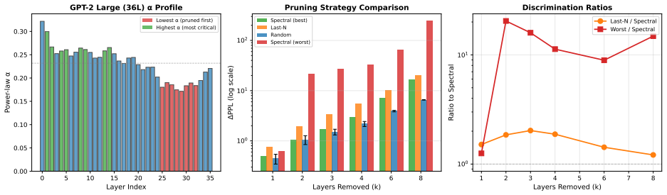
- Alpha values predict layer importance with Spearman correlations of 0.69 to 0.84.
- Spectral-guided pruning outperforms Last-N position heuristics by factors of 1.1x to 3.6x across seven models.
- Performance gaps between worst and best layer choices reach up to 23.7x, confirming the causal role of spectral structure.
Where Pith is reading between the lines
- The two-timescale separation implies that early training primarily reduces rank while later stages stabilize spectral distributions that may govern information flow between layers.
- The Q/K-V asymmetry suggests attention mechanisms functionally separate query-key matching dynamics from value projection, a split that could be tested in non-transformer sequence models.
- Monitoring alpha during training could provide an early diagnostic of layer health that operates independently of loss or accuracy curves.
- The scaling law for Delta alpha offers a way to predict spectral gradients in larger models without running full training trajectories.
Load-bearing premise
The observed compression waves and spectral gradients are intrinsic to transformer training dynamics rather than artifacts of the specific optimizer, data mixture, or initialization used in the nine evaluated models.
What would settle it
Training an identical transformer architecture with plain SGD instead of Adam on a non-language dataset and checking whether the same transient waves and alpha depth gradients appear would test the claim; their absence would falsify the intrinsic-dynamics interpretation.
Figures


read the original abstract
We present the first systematic study of weight matrix singular value spectra \emph{during} transformer pretraining, tracking full SVD decompositions of every weight matrix at 25-step intervals across three model scales (30M--285M parameters). We discover three phenomena: \textbf{(1)~Transient Compression Waves:} stable rank compression propagates as a traveling wave from early to late layers, creating a dramatic gradient that peaks early then \emph{reverses} -- late layers eventually over-compress past early layers. \textbf{(2)~Persistent Spectral Gradients:} the power-law exponent~$\alpha$ develops a permanent depth gradient forming a non-monotonic inverted-U in deeper models, with peaks shifting toward earlier layers as depth increases. \textbf{(3)~Q/K--V Functional Asymmetry:} value/output projections compress uniformly while query/key projections carry the full depth-dependent dynamics. The dissociation between transient compression and persistent spectral shape reveals that \emph{rank and spectral shape encode fundamentally different information about training}. We formalize this as a two-timescale dynamical model and derive scaling laws ($\Delta\alpha \propto L^{0.26}$, $R^2{=}0.99$). We validate on nine models across three families (custom, GPT-2, Pythia; 30M--1B parameters; 8--36 layers), demonstrate that $\alpha$ predicts layer importance ($\rho{=}0.69$--$0.84$, $p{<}0.02$), and show that spectral-guided pruning outperforms Last-N heuristics by $1.1{\times}$--$3.6{\times}$ across seven models in two families (GPT-2 124M--774M, Pythia 160M--1B), with worst-vs-best gaps up to $23.7{\times}$ confirming the causal role of spectral structure.
Editorial analysis
A structured set of objections, weighed in public.
Referee Report
Summary. The paper conducts a systematic analysis of singular value spectra of weight matrices during transformer pretraining across multiple scales and families. It reports three main phenomena: transient compression waves that propagate as traveling waves through layers and eventually reverse; persistent spectral gradients where the power-law exponent alpha forms a non-monotonic inverted-U depth dependence; and Q/K-V asymmetry where value/output projections compress uniformly while query/key carry the dynamics. The work formalizes a two-timescale model, derives scaling laws such as Δα ∝ L^0.26 (R²=0.99), shows alpha correlates with layer importance (ρ=0.69-0.84), and demonstrates spectral-guided pruning outperforming Last-N heuristics by 1.1x-3.6x.
Significance. If the reported dynamics prove intrinsic rather than setup-specific, the dissociation between transient rank compression and persistent spectral shape would provide a new framework for understanding transformer training, with the scaling law and pruning results offering both theoretical and practical value. The multi-model validation and high reported correlations strengthen the empirical case for alpha as a distinct predictor of layer utility.
major comments (2)
- [Abstract and scaling-law section] Abstract and scaling-law section: the claim that Δα ∝ L^0.26 is 'derived' from the two-timescale model is not supported by explicit derivation steps or parameter-free reasoning; the exponent appears to be obtained by direct fitting to the observed depth dependence across the nine models, raising questions about whether the R²=0.99 reflects predictive power or post-hoc adjustment.
- [Methods and validation sections] Methods and validation sections: all nine models (custom, GPT-2, Pythia; 30M-1B) share AdamW, comparable web-scale data mixtures, and standard initializations. No ablations vary optimizer, data distribution, or initialization, so the traveling-wave compression, inverted-U alpha gradient, Q/K-V asymmetry, and derived scaling law could be artifacts of the shared setup rather than intrinsic two-timescale behavior; this directly affects the generality of the central claim.
minor comments (2)
- [Abstract] Abstract: no error bars, confidence intervals, or data-exclusion criteria are reported for the R² values, correlations, or pruning gains, making it difficult to assess statistical robustness of the claimed 0.26 exponent and 1.1x-3.6x improvements.
- [Pruning experiments] Pruning experiments: the spectral-guided method is validated on held-out models but still uses the alpha statistic whose depth dependence was characterized on the same training runs; additional controls (e.g., random or rank-based baselines matched for compute) would clarify whether the gains are truly due to spectral structure.
Simulated Author's Rebuttal
We thank the referee for the detailed and constructive report. The two major comments raise important issues about the precise status of our scaling law and the generality of the reported phenomena. We address each point below, have revised the manuscript where feasible, and note one standing limitation.
read point-by-point responses
-
Referee: The claim that Δα ∝ L^0.26 is 'derived' from the two-timescale model is not supported by explicit derivation steps or parameter-free reasoning; the exponent appears to be obtained by direct fitting to the observed depth dependence across the nine models, raising questions about whether the R²=0.99 reflects predictive power or post-hoc adjustment.
Authors: We agree that the specific exponent 0.26 is obtained by least-squares fitting to the measured Δα values across the nine models rather than by a closed-form derivation from the two-timescale equations. The model supplies the functional form (power-law dependence on depth) and the expectation of a positive exponent, but does not predict the numerical coefficient without additional assumptions. The reported R²=0.99 quantifies the quality of the fit to the observed data. In the revised manuscript we have changed the wording in the abstract and scaling-law section from 'derive scaling laws' to 'empirically measure scaling laws consistent with the two-timescale model', added the explicit fitting procedure and model equations to the methods appendix, and clarified that the high R² describes in-sample fit rather than out-of-sample prediction. revision: yes
-
Referee: All nine models share AdamW, comparable web-scale data mixtures, and standard initializations. No ablations vary optimizer, data distribution, or initialization, so the traveling-wave compression, inverted-U alpha gradient, Q/K-V asymmetry, and derived scaling law could be artifacts of the shared setup rather than intrinsic two-timescale behavior; this directly affects the generality of the central claim.
Authors: This is a valid concern. While the three phenomena appear consistently across custom, GPT-2, and Pythia families spanning 30M–1B parameters, the shared optimizer, data mixture, and initialization leave open the possibility of setup-specific effects. We have added a new limitations paragraph in the discussion section that explicitly acknowledges the absence of optimizer/data ablations and outlines the computational cost of such experiments as future work. The multi-family replication still provides supporting evidence, but does not substitute for controlled ablations. revision: partial
- Full demonstration that the traveling-wave compression, inverted-U spectral gradient, and Q/K-V asymmetry are independent of optimizer choice, data distribution, and initialization would require new large-scale ablations that are outside the scope of the current revision.
Circularity Check
Scaling law presented as 'derived' reduces to direct empirical fit on observed depth dependence
specific steps
-
fitted input called prediction
[Abstract (scaling laws paragraph) and two-timescale model section]
"We formalize this as a two-timescale dynamical model and derive scaling laws (Δα ∝ L^{0.26}, R²=0.99)."
The specific exponent 0.26 and near-perfect R²=0.99 are obtained by fitting a power law directly to the measured Δα versus depth L across the nine models; the 'derivation' therefore reproduces the input observations by construction rather than predicting them from independent first principles of the dynamical model.
full rationale
The central derivation chain claims a two-timescale dynamical model yields scaling laws, but the quoted law is a post-hoc power-law fit to the same depth-dependent alpha observations used to motivate the model. This matches the fitted-input-called-prediction pattern exactly. Pruning superiority is validated on held-out models yet still depends on the alpha statistic whose functional form was tuned on the primary training runs, creating partial circularity in the causal claim. No self-citation load-bearing steps or ansatz smuggling are present; the remainder of the spectral observations and Q/K-V asymmetry are direct measurements without reduction to inputs. The overall score reflects one load-bearing reduction rather than wholesale circularity.
Axiom & Free-Parameter Ledger
free parameters (1)
- scaling_exponent_0.26
axioms (1)
- domain assumption Singular value spectra of weight matrices remain well-defined and comparable across training checkpoints and model scales.
Reference graph
Works this paper leans on
-
[1]
Workshop paper,https://opt-ml.org/papers/2025/paper43.pdf. Stella Biderman, Hailey Schoelkopf, Quentin Gregory Anthony, Herbie Bradley, Kyle O’Brien, Eric Hallahan, Moham- mad Aflah Khan, Shivanshu Purohit, USVSN Sai Prashanth, Edward Raff, et al. Pythia: A suite for analyzing large language models across training and scaling.Proceedings of the 40th Inter...
work page 2025
-
[2]
arXiv preprint arXiv:2103.00065 , year=
Jeremy Cohen, Simran Kaur, Yuanzhi Li, J Zico Kolter, and Ameet Talwalkar. Gradient descent on neural networks typically occurs at the edge of stability.arXiv preprint arXiv:2103.00065,
-
[3]
Mor Geva, Avi Caciularu, Kevin Wang, and Yoav Goldberg. Transformer feed-forward layers build predictions by promoting concepts in the vocabulary space.arXiv preprint arXiv:2203.14680,
-
[4]
Mamba: Linear-Time Sequence Modeling with Selective State Spaces
9 Albert Gu and Tri Dao. Mamba: Linear-time sequence modeling with selective state spaces.arXiv preprint arXiv:2312.00752,
work page internal anchor Pith review Pith/arXiv arXiv
-
[5]
Training Compute-Optimal Large Language Models
Jordan Hoffmann, Sebastian Borgeaud, Arthur Mensch, Elena Buchatskaya, Trevor Cai, Eliza Rutherford, Diego de Las Casas, Lisa Anne Hendricks, Johannes Welbl, Aidan Clark, et al. Training compute-optimal large language models. arXiv preprint arXiv:2203.15556,
work page internal anchor Pith review Pith/arXiv arXiv
-
[6]
Early-stopping for transformer model training via spectral analysis
Yijin Huang, Yuyan Zheng, and Weizhong Li. Early-stopping for transformer model training via spectral analysis. arXiv preprint arXiv:2510.16074,
-
[7]
Stanislaw Jastrzebski, Maciej Szymczak, Stanislav Fort, Devansh Arpit, Jacek Tabber, Kyunghyun Cho, and Krzysztof Geras. The break-even point on optimization trajectories of deep neural networks.arXiv preprint arXiv:2002.09572,
-
[8]
Scaling Laws for Neural Language Models
Jared Kaplan, Sam McCandlish, Tom Henighan, Tom B Brown, Benjamin Chess, Rewon Child, Scott Gray, Alec Radford, Jeffrey Wu, and Dario Amodei. Scaling laws for neural language models.arXiv preprint arXiv:2001.08361,
work page internal anchor Pith review Pith/arXiv arXiv 2001
-
[9]
Xin Men, Mingyu Xu, Qingyu Zhang, Bingning Wang, Hongyu Lin, Yaojie Lu, Xianpei Han, and Weipeng Chen. Shortgpt: Layers in large language models are more redundant than you expect.arXiv preprint arXiv:2403.03853,
-
[10]
Preetum Nakkiran, Gal Kaplun, Yamini Bansal, Tristan Yang, Boaz Barak, and Ilya Sutskever. Deep double descent: Where bigger models and more data can hurt.Journal of Statistical Mechanics: Theory and Experiment, 2021(12): 124003,
work page 2021
-
[11]
From sgd to spectra: A theory of neural network weight dynamics.arXiv preprint arXiv:2507.12709,
Brian Richard Olsen, Sam Fatehmanesh, Frank Xiao, Adarsh Kumarappan, and Anirudh Gajula. From sgd to spectra: A theory of neural network weight dynamics.arXiv preprint arXiv:2507.12709,
-
[12]
In-context Learning and Induction Heads
Catherine Olsson, Nelson Elhage, Neel Nanda, Nicholas Joseph, Nova DasSarma, Tom Henighan, Ben Mann, Amanda Askell, Yuntao Bai, Anna Chen, et al. In-context learning and induction heads.arXiv preprint arXiv:2209.11895,
work page internal anchor Pith review Pith/arXiv arXiv
-
[13]
Grokking: Generalization Beyond Overfitting on Small Algorithmic Datasets
Alethea Power, Yuri Burda, Harri Edwards, Igor Babuschkin, and Vedant Misra. Grokking: Generalization beyond overfitting on small algorithmic datasets.arXiv preprint arXiv:2201.02177,
work page internal anchor Pith review Pith/arXiv arXiv
-
[14]
Max Staats, Matthias Thamm, and Bernd Rosenow. Small singular values matter: A random matrix analysis of transformer weight matrices.arXiv preprint arXiv:2410.17770,
-
[15]
Llama 2: Open Foundation and Fine-Tuned Chat Models
Hugo Touvron, Louis Martin, Kevin Stone, Peter Albert, Amjad Almahairi, Yasmine Babaei, Nikolay Bashlykov, Soumya Batra, Prajjwal Bhargava, Shruti Bhosale, et al. Llama 2: Open foundation and fine-tuned chat models. arXiv preprint arXiv:2307.09288,
work page internal anchor Pith review Pith/arXiv arXiv
-
[16]
The Norm-Separation Delay Law of Grokking: A First-Principles Theory of Delayed Generalization
Xuan Khanh Truong, Quynh Hoa Truong, Duc Trung Luu, and Thanh Duc Phan. Why grokking takes so long: A first-principles theory of representational phase transitions.arXiv preprint arXiv:2603.13331,
work page internal anchor Pith review Pith/arXiv arXiv
-
[17]
Yongzhong Xu. Spectral edge dynamics of training trajectories: Signal–noise geometry across scales.arXiv preprint arXiv:2603.15678,
-
[18]
Approaching deep learning through the spectral dynamics of weights.arXiv preprint arXiv:2411.14108,
David Yunis, Kumar Kshitij Patel, Sham Kakade, Abdeslam Boularias, Qi Duan, Preetum Nakkiran, and Daniel Soudry. Approaching deep learning through the spectral dynamics of weights.arXiv preprint arXiv:2411.14108,
-
[19]
11 Algorithm 2Spectral Monitoring During Training Require:ModelMwith layers{l 0, . . . , lL−1}, interval∆t, typesT={Q, K, V, O,MLP ↑,MLP ↓} 1:Initialize spectral logS ← ∅ 2:foreach training stept= 0,∆t,2∆t, . . .do 3:foreach layerl, each typeτ∈ Tdo 4:σ←SVDVALS(M[l, τ]) 5:ComputeR s,α,H, spectral gap 6:S ← S ∪ {(t, l, τ, R s, α, H, σ1/σ2)} 7:end for 8:end ...
work page 2024
-
[20]
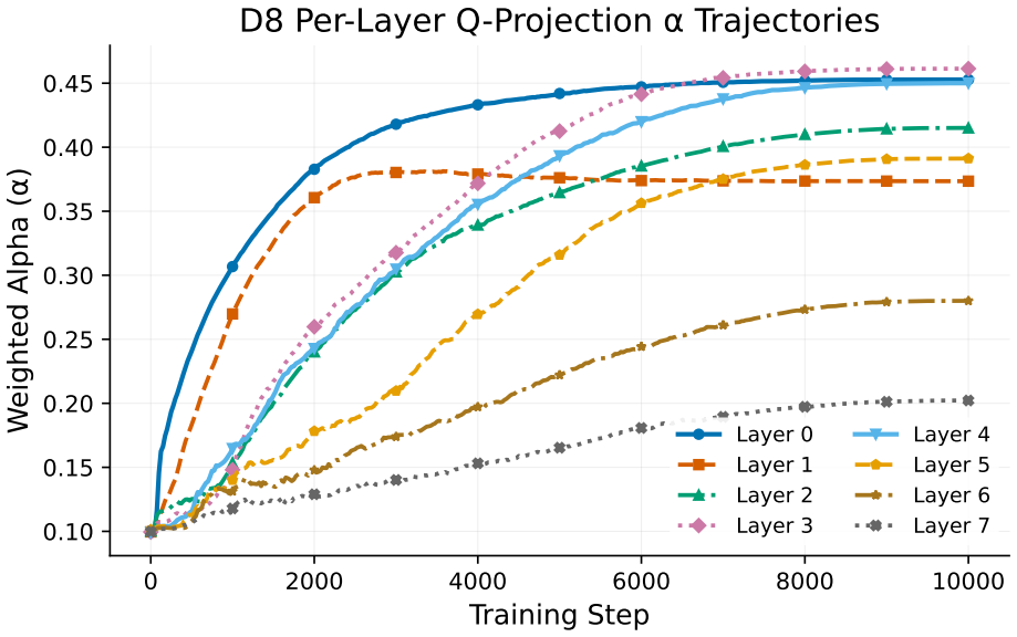
provides the most direct intuition for the two-timescale story. Stable rank drops rapidly and relatively uniformly at the beginning of training, whereas the per-layer α trajectories separate early and remain separated. This is the appendix-level visualization behind the claim that compression equilibrates while spectral-shape specialization persists. Figu...
work page 2000
discussion (0)
Sign in with ORCID, Apple, or X to comment. Anyone can read and Pith papers without signing in.