Trees to Flows and Back: Unifying Decision Trees and Diffusion Models
Pith reviewed 2026-05-22 10:19 UTC · model grok-4.3
The pith
Decision trees and diffusion models correspond mathematically in limiting regimes, revealing a shared Global Trajectory Score Matching optimization principle.
A machine-rendered reading of the paper's core claim, the machinery that carries it, and where it could break.
Core claim
Hierarchical decision trees and diffusion processes are mathematically correspondent in appropriate limiting regimes; this correspondence produces a shared optimization principle called Global Trajectory Score Matching, under which gradient boosting in its idealized form is asymptotically optimal.
What carries the argument
The crisp mathematical correspondence between hierarchical decision trees and diffusion processes in limiting regimes, which makes the Global Trajectory Score Matching principle emerge as the common objective.
If this is right
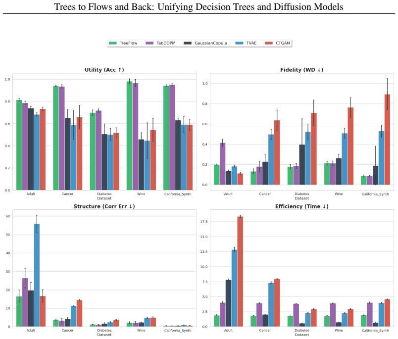
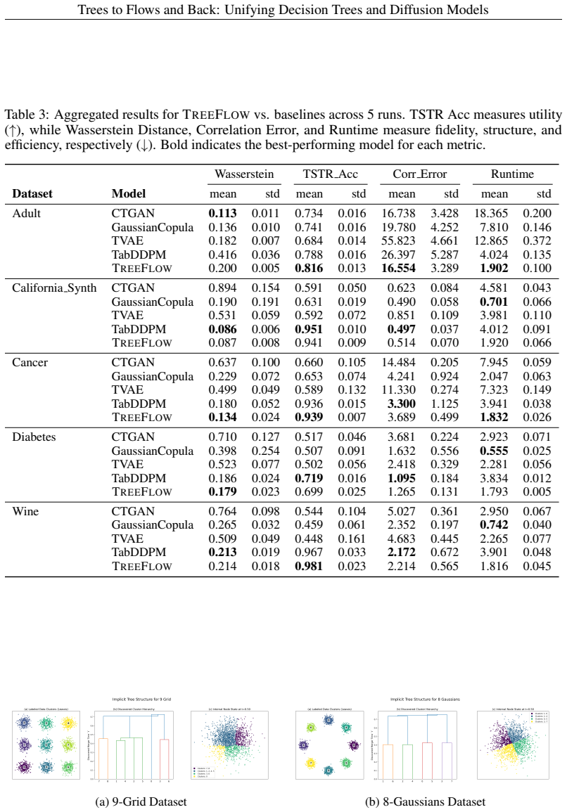
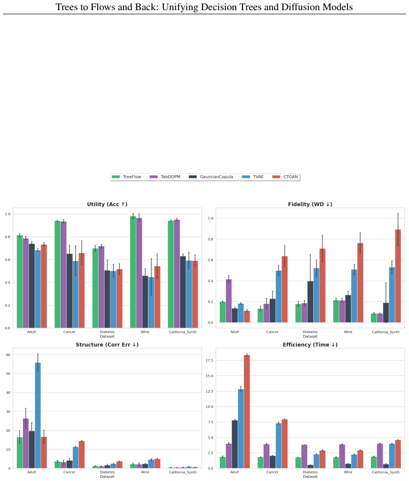
- TreeFlow produces competitive generation quality on tabular data while delivering higher fidelity and roughly 2x computational speedup.
- DSMTree transfers hierarchical decision logic into neural networks and matches the teacher model within 2 percent on many benchmarks.
- Gradient boosting becomes the asymptotically optimal procedure for the shared Global Trajectory Score Matching objective.
- The unification supplies a common lens for analyzing and improving both discrete tree-based and continuous flow-based generative models.
Where Pith is reading between the lines
- Hybrid architectures could alternate between tree splits for interpretability and diffusion steps for smooth sampling on the same trajectory objective.
- The limiting-regime correspondence may extend to other discrete structures such as decision lists or recursive partitioning schemes.
- Practical implementations could test whether enforcing the Global Trajectory Score Matching objective directly improves stability in existing diffusion pipelines.
Load-bearing premise
The mathematical correspondence between hierarchical decision trees and diffusion processes holds in the required limiting regimes.
What would settle it
A direct numerical check showing that the idealized gradient boosting procedure fails to converge to the optimum of Global Trajectory Score Matching when the tree-to-diffusion limit is taken.
Figures
read the original abstract
Decision trees and diffusion models are ostensibly disparate model classes, one discrete and hierarchical, the other continuous and dynamic. This work unifies the two by establishing a crisp mathematical correspondence between hierarchical decision trees and diffusion processes in appropriate limiting regimes. Our unification reveals a shared optimization principle: \emph{Global Trajectory Score Matching (GTSM)}, for which gradient boosting (in an idealized version) is asymptotically optimal. We underscore the conceptual value of our work through two key practical instantiations: \treeflow, which achieves competitive generation quality on tabular data with higher fidelity and a 2\times computational speedup, and \dsmtree, a novel distillation method that transfers hierarchical decision logic into neural networks, matching teacher performance within 2\% on many benchmarks.
Editorial analysis
A structured set of objections, weighed in public.
Referee Report
Summary. The paper claims to establish a crisp mathematical correspondence between hierarchical decision trees and diffusion processes in appropriate limiting regimes. This unification reveals a shared optimization principle called Global Trajectory Score Matching (GTSM), for which an idealized version of gradient boosting is asymptotically optimal. Two practical instantiations are presented: TreeFlow, which generates tabular data with competitive quality, higher fidelity, and 2x speedup, and DSMTREE, a distillation method that transfers decision logic into neural networks while matching teacher performance within 2% on benchmarks.
Significance. If the limiting-regime correspondence and GTSM optimality hold with rigorous support, the work could bridge discrete hierarchical models and continuous generative dynamics in machine learning, offering conceptual unification and new algorithmic tools. The practical methods suggest efficiency gains for tabular generation and model compression, with potential for broader impact if the theoretical foundation is solidified.
major comments (3)
- [Section 3] Section 3 (unification): The mapping of tree depth to diffusion time and leaf probabilities to marginals is presented without an explicit derivation or error analysis showing that the Global Trajectory Score Matching loss remains identical after the continuum limit. The assumption that discrete splitting gradients equate to continuous score-matching gradients requires additional regularity conditions to ensure discretization bias vanishes uniformly; without this, the shared optimization principle does not transfer.
- [Abstract] Abstract and optimality discussion: The assertion that idealized gradient boosting is asymptotically optimal for GTSM lacks derivations, analysis of limiting regimes, or verification details. This raises the risk that the optimality claim reduces to the definitions introduced in the paper's own limiting process rather than following independently.
- [Section 3] Section 3: The crisp correspondence between decision trees and diffusion trajectories is asserted to hold in appropriate limiting regimes, but no analysis addresses whether non-vanishing discretization bias from the splitting process could invalidate the exact equivalence of the GTSM objective.
minor comments (2)
- [Section 3] Clarify notation distinguishing discrete tree quantities from their continuous diffusion counterparts, particularly in equations involving the limiting process.
- [Practical instantiations] Add more detail on empirical verification for the claimed 2x speedup and 2% performance match in the practical sections to support the instantiations.
Simulated Author's Rebuttal
We thank the referee for the detailed and constructive comments, which identify opportunities to strengthen the rigor of our theoretical unification. We address each major comment below and will incorporate revisions to provide the requested derivations and analyses.
read point-by-point responses
-
Referee: [Section 3] Section 3 (unification): The mapping of tree depth to diffusion time and leaf probabilities to marginals is presented without an explicit derivation or error analysis showing that the Global Trajectory Score Matching loss remains identical after the continuum limit. The assumption that discrete splitting gradients equate to continuous score-matching gradients requires additional regularity conditions to ensure discretization bias vanishes uniformly; without this, the shared optimization principle does not transfer.
Authors: We agree that an explicit derivation and error analysis would improve clarity. In the revised manuscript, we will expand Section 3 with a step-by-step derivation of the continuum limit, mapping tree depth to diffusion time and leaf probabilities to marginals. We will also include an error analysis under suitable regularity conditions (e.g., Lipschitz continuity of the underlying densities) demonstrating uniform convergence of the GTSM loss and vanishing discretization bias. This will rigorously establish transfer of the shared optimization principle. revision: yes
-
Referee: [Abstract] Abstract and optimality discussion: The assertion that idealized gradient boosting is asymptotically optimal for GTSM lacks derivations, analysis of limiting regimes, or verification details. This raises the risk that the optimality claim reduces to the definitions introduced in the paper's own limiting process rather than following independently.
Authors: The optimality follows from interpreting boosting steps as a discretization of the gradient flow minimizing the GTSM functional in the continuum limit, independent of the tree-diffusion correspondence. We will revise the abstract and add a subsection with the derivation, limiting-regime analysis, and verification on low-dimensional cases. This grounds the result in standard functional gradient descent theory rather than circularity. revision: yes
-
Referee: [Section 3] Section 3: The crisp correspondence between decision trees and diffusion trajectories is asserted to hold in appropriate limiting regimes, but no analysis addresses whether non-vanishing discretization bias from the splitting process could invalidate the exact equivalence of the GTSM objective.
Authors: We concur that explicit treatment of discretization bias is needed. The revision will add analysis in Section 3 showing that, under bounded splitting criteria and Lipschitz score functions, the bias vanishes as the partition refines and the time discretization step approaches zero. This confirms equivalence of the GTSM objectives in the limit and preserves the correspondence. revision: yes
Circularity Check
No significant circularity in unification or optimality claim
full rationale
The paper presents a mathematical correspondence between hierarchical decision trees and diffusion processes in limiting regimes, from which a shared Global Trajectory Score Matching (GTSM) principle is derived, with an asymptotic optimality statement for idealized gradient boosting. No equations or definitions in the provided abstract or context reduce the claimed optimality or unification to a self-referential fit, renaming, or self-citation chain by construction. The limiting-regime mapping is offered as an independent derivation rather than a tautology, and the work remains self-contained against external benchmarks without load-bearing self-references that collapse the central result.
Axiom & Free-Parameter Ledger
Lean theorems connected to this paper
-
IndisputableMonolith/Foundation/AbsoluteFloorClosure.leanreality_from_one_distinction unclear?
unclearRelation between the paper passage and the cited Recognition theorem.
Theorem 2.3 (Limit under Dyadic Refinement) ... continuous-time filtration {Ft} ... Gt converges to time-invariant generator G
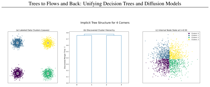
-
IndisputableMonolith/Cost/FunctionalEquation.leanwashburn_uniqueness_aczel unclear?
unclearRelation between the paper passage and the cited Recognition theorem.
Global Trajectory Score Matching (GTSM) ... LC GTSM(θ) = ½ ∫ w(t) E[||sθ−s∗||²D] dt
What do these tags mean?
- matches
- The paper's claim is directly supported by a theorem in the formal canon.
- supports
- The theorem supports part of the paper's argument, but the paper may add assumptions or extra steps.
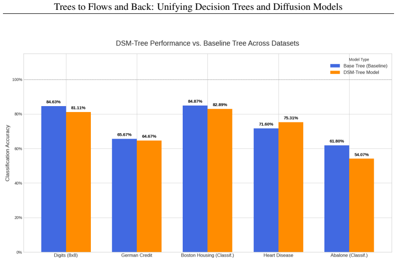
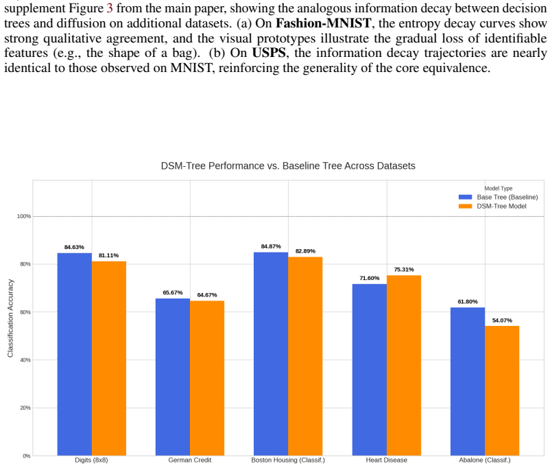
- extends
- The paper goes beyond the formal theorem; the theorem is a base layer rather than the whole result.
- uses
- The paper appears to rely on the theorem as machinery.
- contradicts
- The paper's claim conflicts with a theorem or certificate in the canon.
- unclear
- Pith found a possible connection, but the passage is too broad, indirect, or ambiguous to say the theorem truly supports the claim.
Reference graph
Works this paper leans on
-
[1]
Axiom 1: Measurability (Information Erasure).The output density p(x, k) must not contain information about the boundaries that were erased in the transition from Πk−1. This meansp(x, k)must be measurable with respect to the coarser sigma-algebraF k generated by the partitionΠ k
-
[2]
Axiom 2: Partial Averages (Probability Conservation).The probability mass must be conserved within every region of the new partition. This property must extend to all sets A∈ F k, such that: Z A p(x, k)dx= Z A p(x, k−1)dx∀A∈ F k.(11) A fundamental theorem of measure theory states that for a given function p(x, k−1) and a sigma- algebra Fk, there exists a ...
work page 2019
-
[3]
Consistent convergence:For any t1 < t2, the sequence of propagators {P(n) t2←t1 } converges to a limitP t2←t1
-
[4]
Bounded intermediate complexity:The ”geometric complexity” added at refinement step n, measured by a suitable metric on partitions, isO(2 −n). Then: (i) The limiting process has a generator Gt with local Lipschitz structure on any compact I⊂[0, T]. (ii) For any sequence of compact intervalsIm ↑[0, T] , there exists a subsequence of refinements such that t...
work page 2019
-
[5]
The series terminates after the second term, i.e.,D (n)(x, t)≡0for alln >2
-
[6]
The expansion cannot terminate at any finite order greater than two
The series does not terminate, and all even-ordered momentsD (2m) form≥1are strictly positive. The expansion cannot terminate at any finite order greater than two. Proof. The proof demonstrates that if any moment D(n) for n >2 is non-zero, then moments of arbitrarily high order must also be non-zero. For clarity, we present the proof in one dimension; the...
work page 2004
-
[7]
to truncate exactly after the second term. The remaining n= 1 (drift) and n= 2 (diffusion) terms constitute the Fokker-Planck equation, which describes the evolution of the probability density p(x, t): ∂p(x, t) ∂t =− dX i=1 ∂ ∂xi [fi(x)p(x, t)] + 1 2 dX i,j=1 ∂2 ∂xi∂xj [(g(x)g(x)⊤)ijp(x, t)].(43) Second, we establish the equivalence to the SDE. It is a st...
work page 2004
-
[8]
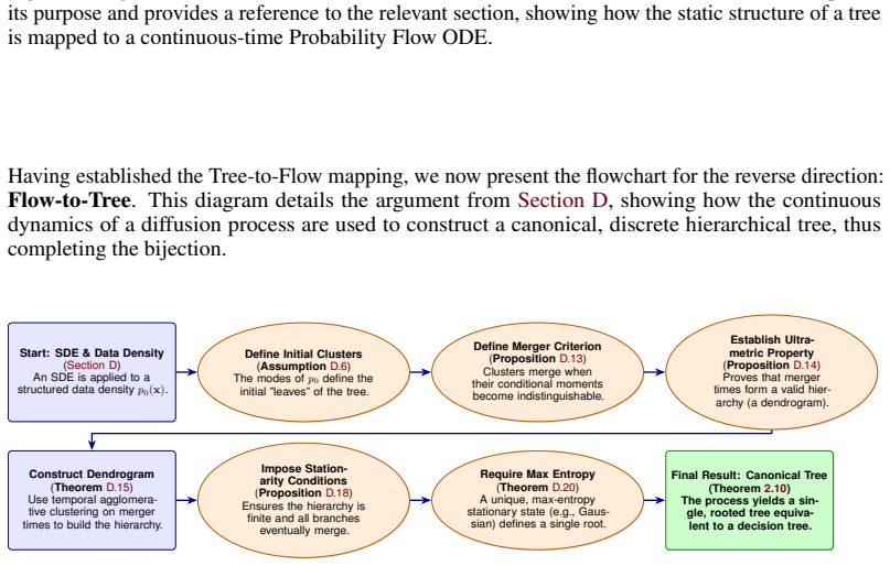
The basins of attraction Bk :={x: lim t→∞ ϕt(x) =x ∗ k} under the gradient flow ˙x= ∇logp 0(x)form a partition ofX,
-
[9]
There existsρ min >0such thatinf x∈∂Bk p0(x)< p 0(x∗ k)−ρ min for allk. Definition D.7(Level-Set Clustering).For a threshold λ∈(0,max k p0(x∗ k)), define the super-level set: Sλ :={x:p 0(x)≥λ}.(45) Theinitial clustersare the connected components of Sλ for λ chosen such that Sλ has exactly K components, one containing each modex ∗ k. Proposition D.8(Well-D...
work page 2025
-
[10]
, CK} are distinct by definition, forming the leaves of our hierarchy
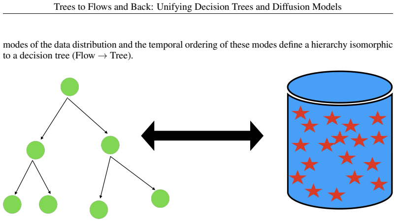
Initialization (Leaves at t= 0 ):At time t= 0 , all K clusters {C1, . . . , CK} are distinct by definition, forming the leaves of our hierarchy
-
[11]
The first merger event occurs at the minimum of these times, t1 = mini,j t(n,ϵ) ij
First Merger:We compute the set of all pairwise merger times, {t(n,ϵ) ij } for i̸=j . The first merger event occurs at the minimum of these times, t1 = mini,j t(n,ϵ) ij . Let this minimum occur for the pair (Ca, Cb). At time t1, we merge Ca and Cb into a new super-cluster, Cab. This event defines the lowest-level branch in the hierarchy
-
[12]
Iterative Merging:We now have a set of K−1 clusters. We repeat the process, computing the merger times between all pairs in this new set (including between the new super-cluster and other original clusters). The next merger event at timet 2 > t1 defines the next branch. This agglomerative process continues, and the ordered sequence of merger times defines...
work page 2009
-
[13]
It is a distribution that has no further structural information to lose
Defining the Root:A maximally entropic distribution, such as a uniform distribution over a manifold X , represents a state of complete information loss relative to that manifold. It is a distribution that has no further structural information to lose. This state acts as the single, common ancestor for all possible paths—the root of the tree. Any partition...
-
[14]
This operator models a pure process of information aggregation, or entropy increase
Consistency with Coarse-Graining:The mapping from a tree to an SDE in Section C is based on a coarse-graining operator defined by conditional expectation. This operator models a pure process of information aggregation, or entropy increase. A forward diffusion process is only guaranteed to be a pure entropy-increasing process fromanyinitial state if its st...
work page 2012
-
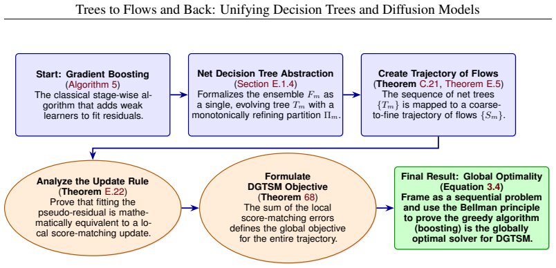
[15]
Partition:Its partition of the feature space, Πm, is thecommon refinementof the partitions induced by all constituent weak learners {h1, . . . , hm}. That is, a region R∈Π m is the largest possible connected subset of X such that for any two points xa,x b ∈R , hi(xa) =h i(xb)for alli∈ {1, . . . , m}
-
[16]
Leaf Values:The value assigned to any leaf region in Πm is the sum of the predictions from all constituent trees,Pm i=1 ηhi(x), whereηis the learning rate. This abstraction provides a monolithic, non-additive representation of the ensemble, allowing us to rigorously analyze the evolution of its decision boundaries as a single geometric object. E.1.3 Monot...
-
[17]
Leaf Partition:The set of its leaf nodes corresponds exactly to the regions of the partition Πm
-
[18]
Hierarchical Structure:The tree’s internal structure is defined by the unique, nested sequence of partitions generated by the boosting algorithm itself: {Π0,Π 1, . . . ,Πm}. The coarsening from the leaves ( Πm) to the root ( Π0 ={X } ) is defined by reversing the historical refinement process. The parent of a node in partition level Πk is the unique regio...
work page 2019
-
[19]
In the context of a diffusion process, this fine-grained information corresponds to the behavior at earlier times. Therefore, the modelSm+1, being more refined, provides a law Pm+1 that is a faithful approximation of the ideal law P⋆ on a larger tail σ-algebra than Sm can. Let us formalize this. For each model Sm, let tm be the earliest time for which its...
-
[20]
Greedy stage-wise algorithms(e.g., boosting, matching pursuit): By construction, Lk is optimized beforeL k+1 is considered
-
[21]
Hierarchical architectures(e.g., progressive growing, curriculum learning): The model capacity for finer scales is introduced only after coarser scales are learned
-
[22]
Spectral bias in neural networks(empirical): Implicit regularization causes neural net- works to learn low-frequency (coarse) components faster than high-frequency (fine) compo- nents (Rahaman et al., 2019). RemarkE.15 (Falsifiability).This assumption can be tested empirically by measuring τk via the learning curves ofL k(θt). For boosting, it holds by de...
work page 2019
-
[23]
Its task is to find an operatorR ⋆ m+1 that transitionsS ⋆ m to a modelS ⋆ m+1 ∈K ⋆ tm+1
The structurally-supervised learner knows the next target class is K ⋆ tm+1. Its task is to find an operatorR ⋆ m+1 that transitionsS ⋆ m to a modelS ⋆ m+1 ∈K ⋆ tm+1
-
[24]
The data-supervised learner (boosting) does not know the target class K ⋆ tm+1. It uses the local data supervision (residuals) to find an update h⋆ m+1 that produces a new model Sm+1
- [25]
-
[26]
The assumption guarantees that the optimal, data-supervised update h⋆ m+1 will be precisely the one that resolves this coarsest remaining part of the problem. By doing so, it produces a new modelS m+1 whose law now correctly matches the ideal law on the tail-fieldF ≥tm+1
-
[27]
Since the update is optimal, it must be the optimal such model,S ⋆ m+1
By definition, any such model is a member of the equivalence classK ⋆ tm+1. Since the update is optimal, it must be the optimal such model,S ⋆ m+1. Therefore, Sm+1 =S ⋆ m+1. By the principle of induction, the trajectories are identical. This crucial equivalence justifies our use of the DSM mathematical machinery to analyze the local, data-supervised boost...
work page 1982
-
[28]
Let X⋆ t be a path generated by the ideal process SDE ⋆, and let Xm,t be a path generated by our model Sm. A core assumption of the score-based modeling framework is that the forward process, defined by drift b(x, t) and diffusion tensor D(x, t), is a fixed, known process independent of the data. The learning task is to find the correct score function to ...
-
[29]
Let X ⋆ τ and Xm,τ be the corresponding reverse-time processes, using the reverse time variable τ∈[0, T] . We consider their evolution starting from the same point at τ= 0 (forward time t=T ), i.e., X ⋆ 0 = Xm,0 =X T . The endpoints of these processes at reverse timeτ=Tare X ⋆ T and Xm,T
-
[30]
We express the endpoints in integral form. The difference between the endpoints is: X ⋆ T −Xm,T = Z T 0 b⋆ rev(X ⋆ τ , τ)−b rev,m(Xm,τ , τ) dτ+ Z T 0 σ(X ⋆ τ , τ)dW ⋆ τ − Z T 0 σ(Xm,τ , τ)dWm,τ . We now take the expectation conditioned on the starting pointXT . The expectation of the stochastic integral terms is zero because Ito integrals are martingales ...
-
[31]
The forward drift terms −b cancel, leaving only the score-dependent terms
We substitute the general formula for the reverse drifts. The forward drift terms −b cancel, leaving only the score-dependent terms. We also change the integration variable back to forward timet=T−τ, which meansdτ=−dtand the integration limits flip. E[X ⋆ T − Xm,T |XT ] =E Z 0 T (D(X⋆ t , t)s⋆ t (X⋆ t )−D(X m,t, t)sm,t(Xm,t)) (−dt) XT =E "Z T 0 (D(X⋆ t , ...
-
[32]
Now we use the crucial fact that Sm ∈K tm. This means that for t≥t m, the law of the model process is a good approximation of the ideal law, Pm|F≥tm ≈P ⋆|F≥tm . This implies that the paths and the score functions are approximately equal in expectation in this range: E[Dsm,t]≈E[Ds ⋆ t ]. The error is negligible for t≥t m. The integrand is therefore effecti...
-
[33]
Finally, we connect this quantity to the expected residual of the boosting algorithm. The expected residual at stepm+ 1is taken over the true data distributionp ⋆ 0(x, y): E[rm+1] =E (x,y)∼p⋆ 0[y−F m(x)]. We analyze the two terms on the right-hand side separately using the law of total expectation
-
[34]
The expected residual at stepm+ 1over the empirical data distribution is: E(x,y)∼pemp 0 [rm+1] =E[y]−E[F m(x)],(60) where the expectations are over the empirical distributionp emp 0 = 1 N PN i=1 δ(xi,yi)
-
[35]
The endpoint of the ideal reverse process, X ∗ T , has lawp ∗
The empirical mean E[y] = 1 N PN i=1 yi is an unbiased estimator of the true target mean. The endpoint of the ideal reverse process, X ∗ T , has lawp ∗
-
[36]
44 Trees to Flows and Back: Unifying Decision Trees and Diffusion Models
Therefore: Epemp 0 [y] =E p∗ 0[X ∗ T ] +O p(N −1/2),(61) whereO p(N −1/2)is the standard Monte Carlo error. 44 Trees to Flows and Back: Unifying Decision Trees and Diffusion Models
-
[37]
The model prediction Fm(x) is the leaf value assigned by the net decision tree Tm. By con- struction, Fm(x) is the conditional expectation under the model’s induced joint distribution: Fm(x) =E y∼pm,0[y|x].(62) The unconditional expectation of the model’s predictions over the empirical feature distribu- tion is: Ex∼pemp 0 [Fm(x)] = 1 N NX i=1 Fm(xi).(63) ...
-
[38]
The key approximation relates these two expectations. Define the distribution mismatch: ∆m :=E x∼pemp 0 [Fm(x)]− Z Fm(x)p m,0(x)dx.(65) We decompose this into two error sources: ∆m = Ex∼pemp 0 [Fm(x)]−E x∼p∗ 0[Fm(x)] | {z } Sampling errorϵ samp + Ex∼p∗ 0[Fm(x)]−E x∼pm,0[Fm(x)] | {z } Model errorϵ model .(66) Sampling error bound:By the central limit theor...
-
[39]
Combining the bounds from (61) and the analysis above: E[rm+1] =E[y]−E[F m(x)]≈E[ X ⋆ T ]−E[ Xm,T ] =E[ X ⋆ T − Xm,T ]. Therefore, the expected residual is anasymptotically unbiased estimatorof the integrated score error, with the bias vanishing asN→ ∞andD KL(p∗ 0∥pm,0)→0. Corollary E.25(Conditions for Exact Equivalence).The meta-score equals the integrat...
-
[40]
The model class contains the true conditionalE[y|x](realizability),
-
[41]
The boosting algorithm has converged:D KL(p∗ 0∥pm,0)< ϵfor arbitrarily smallϵ >0. In practice, the approximation quality is controlled by the sample size N and the residual variance at stepm. 45 Trees to Flows and Back: Unifying Decision Trees and Diffusion Models E.4 Global Optimality of the Greedy Trajectory We have proven that each step of the gradient...
work page 1996
-
[42]
Base Case (m=M−1 ):At the final stage, the decision is to choose hM to transition from state SM−1 . The optimal cost-to-go is simply the minimum possible cost at this stage, as there are no future costs: VM−1(SM−1) = min hM ∈AϵM−1 C(S M−1 , hM). The optimal action, π⋆ M−1(SM−1), is by definition the greedy choice that minimizes this immediate cost
-
[43]
Inductive Hypothesis:Assume that for all steps k > m , the optimal policy π⋆ k is the greedy policy. 3.Inductive Step (m):The Bellman equation for the optimal cost-to-go at stepmis: Vm(Sm) = min hm+1∈A [C(S m, hm+1) +V m+1(T(S m, hm+1))]. Over the finite action spaceA ϵm, the minimum in the Bellman equation is well-defined: Vm(Sm) = min hm+1∈Aϵm [C(S m, h...
work page 2025
-
[44]
The base treeThas bounded depthD <∞and bounded number of leavesL=O(2 D)
-
[45]
The feature space is bounded:∥x∥ ≤Bfor allx∈ X
-
[46]
The loss functionℓ CE isG-Lipschitz continuous in the model parameters. Theorem G.5(Finite-Sample Convergence of DSM-TREE).UnderAssumptionG.4, let ˆθT be the parameters obtained after T gradient descent steps with learning rate η=O(1/ √ T) and batch size B. Then with probability at least1−δ: LDSM(ˆθT )− L DSM(θ∗)≤O D· p dlog(L/δ)√ BT ! ,(79) whereθ ∗ is t...
work page 2018
-
[47]
The data distributionp data(x, y)has bounded support:∥x∥ ≤Bfor allx∈supp(p data)
-
[48]
The base treeThas depthDandL=O(2 D)leaves, with balanced partitioning (each leaf has comparable probability mass)
-
[49]
The velocity networkv θ isG-Lipschitz continuous inxandθ
-
[50]
The path encoding p=PathEncoder(T,x) is deterministic and has bounded norm: ∥p∥ ≤ P. Theorem H.3(Finite-Sample Convergence of TREEFLOW).UnderAssumptionH.2, let ˆθS be the parameters obtained after S gradient descent steps with learning rate η=O(1/ √ S) and batch size B. Then with probability at least1−δ: LTREEFLOW (ˆθS)− L TREEFLOW (θ∗)≤O p d·L·log(L/δ)√ ...
work page 2018
-
[51]
Sampling B data points and computing their path encodings: O(B·D) (traversing tree to depthD)
-
[52]
Sampling noisex (0) and timet:O(B·d)
-
[53]
Computing interpolationsx (t):O(B·d)
-
[54]
Forward pass through velocity network:O(B·C net)
-
[55]
Computing loss and gradients:O(B·d)
-
[56]
Backward pass and parameter update:O(B·C net) The dominant terms are the path encoding (which requires O(D) traversal per sample) and the network forward-backward passes. For a network with hidden dimension h, Cnet =O(d·h+K·h) whereKis the path encoding dimension (typicallyK=Lfor full decision path representation). Multiplying bySsteps and simplifying: O(...
-
[57]
DSM-TREEsolves CGTSM for discriminative modeling: learn the coarse-to-fine trajectory of decision boundaries that minimizes classification error
-
[58]
TREEFLOWsolves CGTSM for generative modeling: learn the coarse-to-fine trajectory of distributions that minimizes generation error (Wasserstein distance). 60 Trees to Flows and Back: Unifying Decision Trees and Diffusion Models Both achieve this by explicitly modeling the hierarchical structure encoded in decision trees as a trajectory through tail-equiva...
work page 2023
-
[59]
Initialize Clusters:The process begins with each of the K ground-truth data classes corresponding to a distinct, active cluster at timet= 0
-
[60]
This is not the simple analytical forward process used for training
Simulate Learned Forward SDE:For each initial cluster, we simulate its evolution forward in time from t= 0 to t=T . This is not the simple analytical forward process used for training. Instead, we use a discretized Euler-Maruyama scheme to solve thelearned forward SDE, where the drift at each step is determined by the model’s own score function: flearned(...
-
[61]
This yields a full trajectory for each cluster’s mean and variance over time
Track Centroid Trajectories:During the simulation, for each cluster and at each time step ti, we compute and store two quantities: the geometric centroid of the cluster’s points and their average spread (mean distance from the centroid). This yields a full trajectory for each cluster’s mean and variance over time
-
[62]
It iterates until only one cluster remains
Iterative Merge Search:The algorithm proceeds via agglomerative clustering. It iterates until only one cluster remains. In each iteration, it searches for the next merge event by checking every possible pair of currently active clusters to find which pair becomes indistinguishable at the earliest future time
-
[63]
This criterion signifies the moment their probability distributions have substantially overlapped
Merge Criterion:Two clusters are defined as ”merged” at the first time step ti where the Euclidean distance between their centroids becomes smaller than the sum of their spreads. This criterion signifies the moment their probability distributions have substantially overlapped
-
[64]
Dendrogram Construction:The pair of clusters with the minimum merge time is formally merged into a new, larger cluster. The event comprising the two original cluster IDs, the merge time ti, and the number of original leaves in the new cluster, is recorded. This sequence of recorded merge events directly forms the linkage matrix for the dendrogram, where t...
work page 1998
-
[65]
Teacher Model Generation:An oracle RandomForestClassifier (100 estimators, depth
-
[66]
is trained. A single DecisionTreeClassifier (depth 15), which serves as our ”Base Tree” baseline, is then trained on the pseudo-labels from this oracle
-
[67]
DSM-TREETraining:A ConditionalSplitModel is trained. This network uses an embedding layer for the tree level j (embedding dim=32) and a 2-hidden-layer MLP (256 units each, with ReLU and BatchNorm) to predict the split decision. It is trained for 30,000 steps (batch size 256) using Adam with a learning rate of10 −3
-
[68]
Inference:To make a prediction, the DSM-TREEmodel is queried iteratively from level j= 0to simulate traversal down the tree until a leaf is reached. ResultsThe detailed performance metrics are provided in Table 2 with a magnified visualization in Figure 14. The results demonstrate that the DSM-TREEmodel, a fully differentiable neural network, can successf...
work page 2016
-
[69]
Tree Encoder:A DecisionTreeClassifier (depth 10) is trained. A TreePathEncoder class converts the decision path of any sample into a sparse vector encoding, where the value at an index is the inverse of the node’s depth
-
[70]
TREEFLOWModel:The model is a conditional MLP that takes as input (x, t,p, y) and outputs a velocity. It uses embeddings for y (embedding dim=16) and a 2-hidden-layer MLP (512 units each, with SiLU and LayerNorm). It is trained for 1000 steps using AdamW (lr= 10 −3) on the conditional flow matching MSE loss. 3.Generation:We provide a target class labelyand...
discussion (0)
Sign in with ORCID, Apple, or X to comment. Anyone can read and Pith papers without signing in.