PDEInvBench: A Comprehensive Dataset and Design Space Exploration of Neural Networks for PDE Inverse Problems
Pith reviewed 2026-06-29 22:39 UTC · model grok-4.3
The pith
Neural networks recover PDE parameters most accurately with two-stage training on parameters then PDE residual fine-tuning.
A machine-rendered reading of the paper's core claim, the machinery that carries it, and where it could break.
Core claim
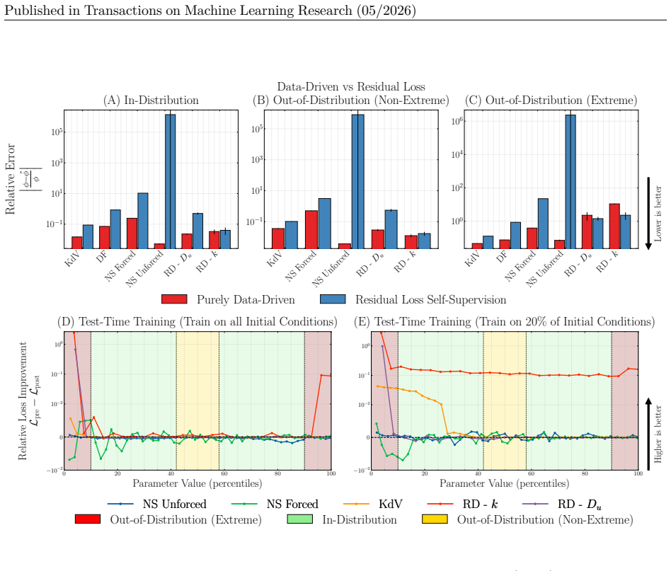
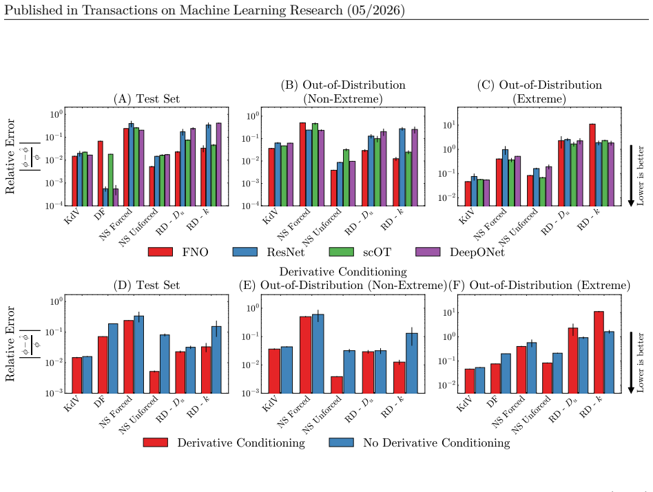
The central claim is that a two-stage procedure—supervised pre-training on PDE parameters followed by test-time fine-tuning that minimizes the PDE residual—combined with derivative features as inputs and training data that emphasizes initial-condition diversity, produces the highest accuracy for neural networks solving PDE inverse problems on both in-distribution and out-of-distribution splits of the new benchmark.
What carries the argument
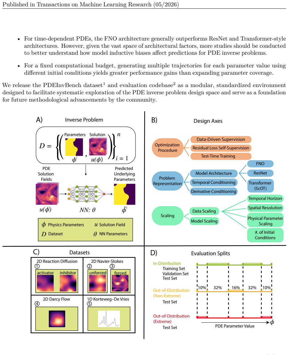
PDEInvBench dataset of simulated solution fields paired with parameters, equipped with in- and out-of-distribution evaluation splits, used to benchmark neural network performance across optimization, representation, and scaling choices.
If this is right
- Models trained under the two-stage schedule should be adopted as the default baseline for neural PDE parameter estimation.
- Input channels should routinely include spatial and temporal derivatives of the observed fields.
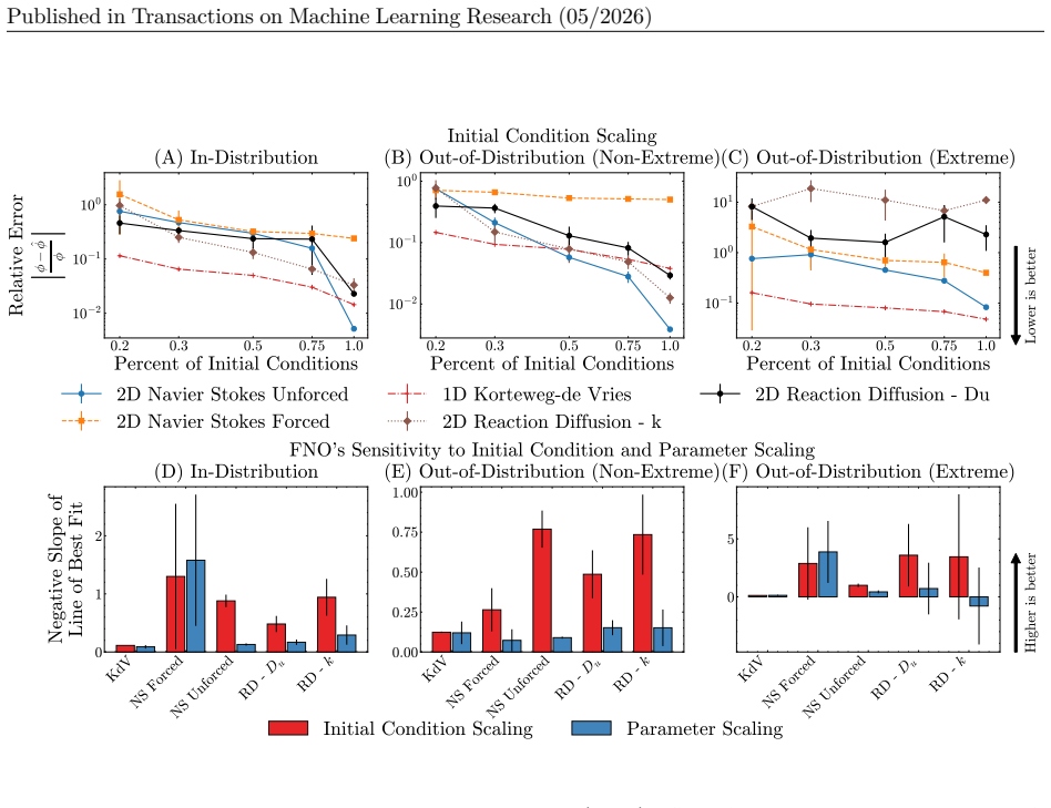
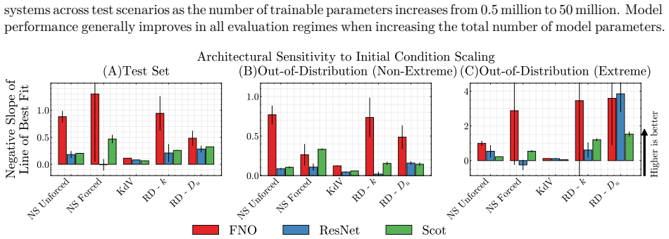
- Data collection efforts should allocate more resources to sampling varied initial conditions than to sampling wider parameter intervals.
- Test-time residual fine-tuning can be expected to close a measurable fraction of the gap between supervised performance and the theoretical optimum.
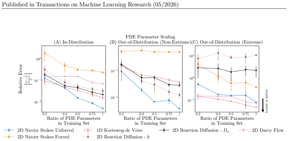
- Scaling laws for these tasks will show larger returns from data diversity than from parameter-range expansion.
Where Pith is reading between the lines
- The same two-stage recipe may transfer to inverse problems outside PDEs, such as recovering coefficients in integral equations or stochastic processes.
- The benchmark could be used to test whether the observed ranking of methods persists when measurement noise levels or missing data patterns match those in actual experiments.
- Practitioners could combine the dataset with transfer-learning protocols to initialize models for new PDE families without regenerating large simulation libraries.
Load-bearing premise
The numerical simulations that generate the dataset correctly capture the true solution behavior of the PDEs under the selected parameters, initial conditions, and boundary conditions.
What would settle it
A controlled experiment on real laboratory or field measurements of a PDE-governed system in which the recommended two-stage training plus derivative inputs fails to outperform plain supervised training on held-out parameter recovery error.
Figures
read the original abstract
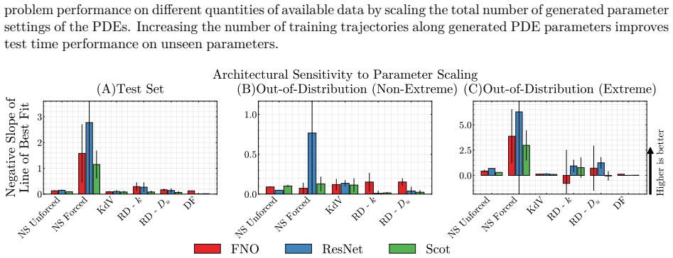
Inverse problems in partial differential equations (PDEs) involve estimating the physical parameters of a system from observed spatiotemporal solution fields. Neural networks are well-suited for PDE parameter estimation due to their capability to model function-to-function space transformations. While existing benchmarks of machine learning methods for PDEs primarily focus on the forward problem, there are no similar comprehensive studies and benchmark datasets on PDE inverse problems, i.e., mapping solution fields to underlying physical parameters. We fill this gap by introducing PDEInvBench, a comprehensive benchmark dataset consisting of numerical simulations for both time-dependent and time-independent PDEs across a wide range of physical behaviors and parameters. Our dataset includes evaluation splits that assess performance in both in-distribution and various out-of-distribution settings. Using our benchmark dataset, we comprehensively explore the design space of neural networks for PDE inverse problems along three key dimensions: (1) optimization procedures, analyzing the role of supervised, self-supervised, and test-time training objectives on performance, (2) problem representations, where we study the value of architectural choices with different inductive biases and various conditioning strategies, and (3) scaling, which we perform with respect to both model and data size. Our experiments reveal several practical insights: 1) neural networks perform best with a two-stage training procedure: initial supervision with PDE parameters followed by test-time fine-tuning using the PDE residual, 2) incorporating PDE derivatives as input features consistently improves accuracy, and 3) increasing the diversity of initial conditions in the training data yields greater performance gains than expanding the range of PDE parameters. We make our dataset and codebase publicly available.
Editorial analysis
A structured set of objections, weighed in public.
Referee Report
Summary. The manuscript introduces PDEInvBench, a benchmark dataset of numerical simulations for PDE inverse problems (time-dependent and time-independent) with in- and out-of-distribution splits. It explores neural network design along three axes—optimization (supervised/self-supervised/test-time objectives), representations (architectures and conditioning), and scaling (model/data size)—and reports three empirical insights: two-stage training (parameter supervision followed by PDE-residual test-time fine-tuning) is best, PDE derivatives as input features improve accuracy, and diverse initial conditions yield larger gains than wider PDE parameter ranges. Dataset and codebase are released publicly.
Significance. If the underlying simulations are faithful, the work supplies a needed public benchmark for PDE inverse problems (a gap relative to forward-problem benchmarks) and supplies concrete, actionable guidance on training procedures, input features, and data diversity. The public release of data and code is a clear strength that supports reproducibility and follow-on research.
major comments (1)
- [abstract / dataset construction paragraph] Abstract / dataset-construction paragraph: the performance deltas supporting the three listed insights rest on numerical solution fields whose fidelity is not verified by convergence studies, grid-refinement checks, or cross-solver comparisons. Without such evidence the reported gains (two-stage training, derivative features, IC diversity) could partly reflect solver-specific discretization artifacts rather than genuine PDE-inverse behavior.
Simulated Author's Rebuttal
We thank the referee for the constructive feedback on the fidelity of the numerical simulations. We address the single major comment below.
read point-by-point responses
-
Referee: [abstract / dataset construction paragraph] Abstract / dataset-construction paragraph: the performance deltas supporting the three listed insights rest on numerical solution fields whose fidelity is not verified by convergence studies, grid-refinement checks, or cross-solver comparisons. Without such evidence the reported gains (two-stage training, derivative features, IC diversity) could partly reflect solver-specific discretization artifacts rather than genuine PDE-inverse behavior.
Authors: We agree that explicit verification of numerical fidelity is important for a benchmark dataset. The simulations were produced with standard, widely used solvers and discretizations drawn from established PDE literature, with resolutions chosen to match common practice for each equation. Because all neural-network variants were evaluated on identical simulation data, any fixed discretization artifacts affect every method equally; the reported relative gains (two-stage training, derivative inputs, IC diversity) therefore reflect differences in how the networks exploit the data rather than solver-specific effects. Nevertheless, to strengthen the manuscript we will add a new subsection to the dataset-construction section that includes grid-refinement studies and limited cross-solver comparisons for representative PDEs, confirming that the chosen discretizations are in the convergent regime. revision: yes
Circularity Check
Empirical benchmark study with no circular derivation chain
full rationale
The paper introduces a synthetic dataset of PDE simulations and reports experimental results on neural network performance for inverse problems. The three main insights (two-stage training, derivative features, IC diversity) are direct empirical measurements on held-out splits of that dataset; no equations, fitted parameters, or predictions are defined in terms of themselves or reduced by construction to the training inputs. No self-citation chains, uniqueness theorems, or ansatzes are invoked as load-bearing steps. The work is self-contained as a benchmark exploration and does not claim any first-principles derivation that collapses to its own data generation procedure.
Axiom & Free-Parameter Ledger
Reference graph
Works this paper leans on
-
[1]
URLhttps://openreview.net/forum?id=wNBARGxoJn
ISSN 2835-8856. URLhttps://openreview.net/forum?id=wNBARGxoJn. Y. Du and A. Krishnapriyan. Eddyformer: Accelerated neural simulations of three-dimensional turbulence at scale. In D. Belgrave, C. Zhang, H. Lin, R. Pascanu, P. Koniusz, M. Ghassemi, and N. Chen, editors,Advances in Neural Information Processing Systems, volume 38, pages 103372–103403. Curran...
-
[2]
doi: 10.1073/pnas.2101784118. URLhttps://www.pnas.org/doi/abs/10.1073/pnas.2101784118. _eprint: https://www.pnas.org/doi/pdf/10.1073/pnas.2101784118. G. Kohl, L.-W. Chen, and N. Thuerey. Benchmarking Autoregressive Conditional Diffusion Mod- els for Turbulent Flow Simulation.arXiv, 2023. doi: 10.48550/arXiv.2309.01745. URL https://doi.org/10.48550/arXiv.2...
-
[3]
The downsampler output is flattened and fed into an MLP head with one hidden layer of 64 units using ReLU activation
Thus, the downsampler reduces the spatial resolution by a factor of 16. The downsampler output is flattened and fed into an MLP head with one hidden layer of 64 units using ReLU activation. A single value is returned, corresponding to the PDE parameter. DeepONet.Our DeepONet implementation follows the standard branch-truck decomposition with slight change...
2026
-
[4]
Initial condition scaling: We vary the number of initial conditions per parameter value at {20%, 35%, 50%, 75%, and 100%} of the full dataset
-
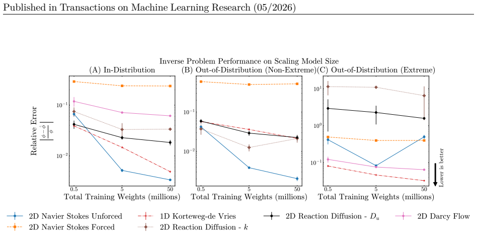
[5]
Parameter scaling: We vary the density of parameter sampling at {20%, 35%, 50%, 75%, and 100%} of the full range
-
[6]
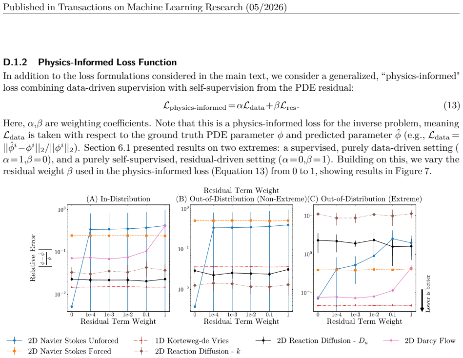
physics-informed
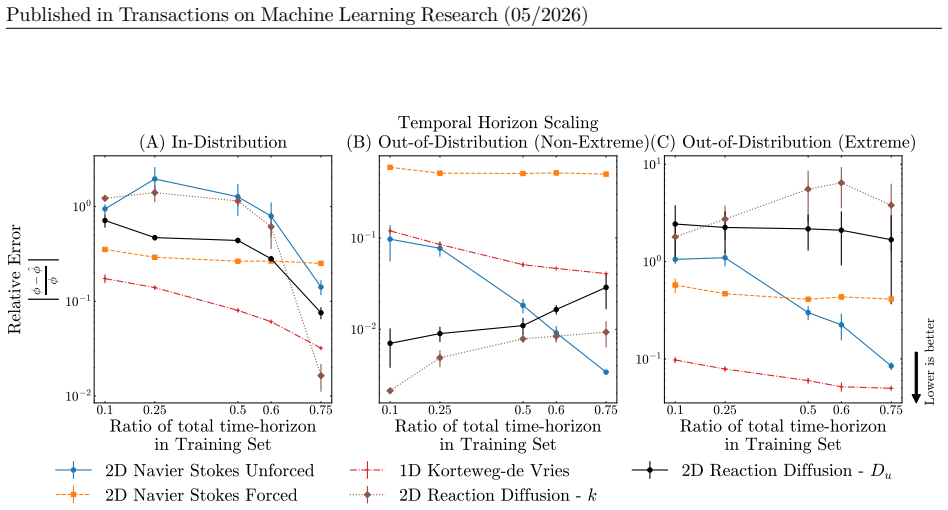
Temporal scaling: We vary the total temporal horizon on which the model is trained by varying the sampled frames from the first {10%, 20%, 50%, 75%} of the total generated temporal range of our dataset. The evaluation set is the final 25% of the generated temporal range for the in-distribution test setting and the entire temporal trajectory for the OOD ev...
2026
-
[7]
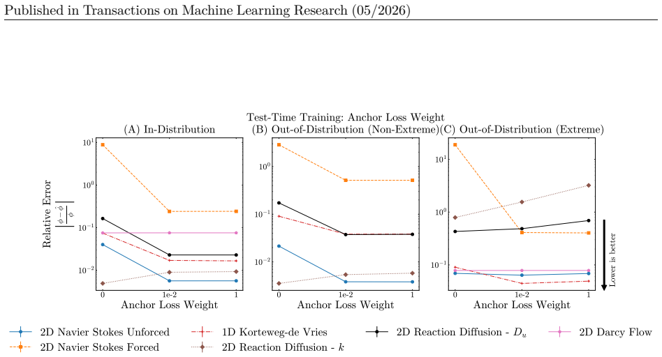
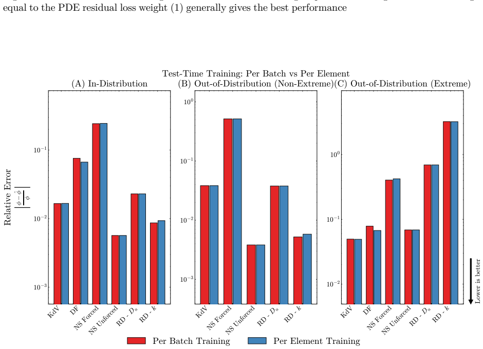
We find that the optimal setting uses equal weighting between residual and anchor terms
influences performance. We find that the optimal setting uses equal weighting between residual and anchor terms. When the anchor loss is weighted too lightly, the relative error tends to increase with training steps, indicating optimization instability. D.1.4 Per-element vs per-batch tailoring We compare performing TTT on aper-elementbasis (batch size of ...
-
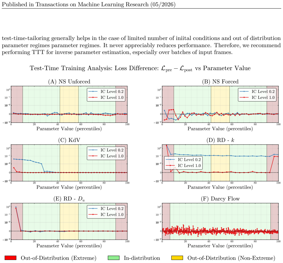
[8]
with anchor loss weights of 1 and show results in Figure 9. TTTper-batchgenerally perform the sameper-samplein all evaluation settings. D.1.5 Test Time Tailoring Comparison with varying levels of ICs We compare the performance of test-time training on models trained on 20% of total available initial conditions and 100% of initial conditions by system in F...
discussion (0)
Sign in with ORCID, Apple, or X to comment. Anyone can read and Pith papers without signing in.