Unveiling Multi-regime Patterns in SciML: Distinct Failure Modes and Regime-specific Optimization

Haiquan Lu; Michael W. Mahoney; Pu Ren; Tianyu Pang; Xiaokun Zhong; Xiaopeng Wang; Yaoqing Yang; Yuanzhe Hu; Yujun Yan; Yuxin Wang

arxiv: 2605.29153 · v1 · pith:JESONGUVnew · submitted 2026-05-27 · 💻 cs.LG · cs.AI· physics.comp-ph

Unveiling Multi-regime Patterns in SciML: Distinct Failure Modes and Regime-specific Optimization

Yuxin Wang , Yuanzhe Hu , Xiaokun Zhong , Xiaopeng Wang , Haiquan Lu , Tianyu Pang , Michael W. Mahoney , Yujun Yan

show 2 more authors

Pu Ren Yaoqing Yang

This is my paper

Pith reviewed 2026-06-29 13:14 UTC · model grok-4.3

classification 💻 cs.LG cs.AIphysics.comp-ph

keywords SciMLtraining regimesphysics-informed neural networksneural operatorsneural ODEsloss-landscape geometryoptimization methodsfailure modes

0 comments

The pith

SciML models exhibit a consistent three-regime structure in training with regime-specific optimization needs.

A machine-rendered reading of the paper's core claim, the machinery that carries it, and where it could break.

The paper seeks to establish that scientific machine learning models enter one of three distinct training regimes depending on hyperparameters, with consistent patterns within each regime. This structure is observed across physics-informed neural networks, neural operators, neural ordinary differential equations, various constraints, and optimizers using a diagnostic framework. The framework examines performance metrics, training dynamics, and loss-landscape geometry simultaneously. Recognizing these regimes matters because it accounts for why optimization methods succeed or fail in different cases and offers a way to develop more robust training procedures for solving differential equations.

Core claim

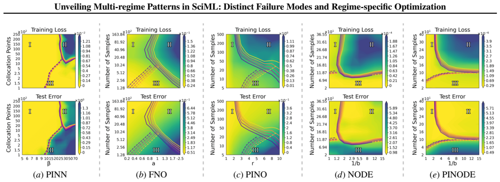
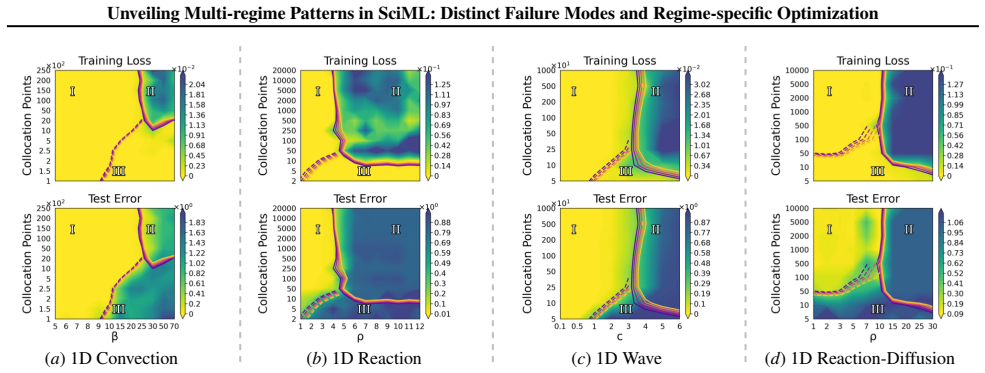
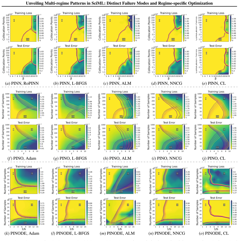
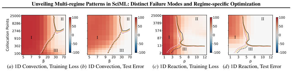
A consistent three-regime structure emerges across many standard SciML models, different constraint enforcements, and various optimizer designs. Optimization effectiveness is regime-specific, with no single method performing well across all regimes. SciML models can exhibit fine-grained failure modes that can challenge conventional interpretations of standard loss-landscape metrics. These results provide an approach to establish a unified, task-oblivious perspective on failure modes in SciML and to inform regime-aware guidance for improving robustness.

What carries the argument

The regime-aware diagnostic framework that jointly analyzes performance, training dynamics, and loss-landscape geometry.

If this is right

No single optimization method performs well across all three regimes.
Optimization must be chosen or adapted based on the identified regime.
Fine-grained failure modes exist beyond what standard loss-landscape metrics reveal.
The three-regime pattern holds for physics-informed neural networks, neural operators, and neural ODEs on ODE and PDE benchmarks.

Where Pith is reading between the lines

These are editorial extensions of the paper, not claims the author makes directly.

Regime detection could be integrated into training loops to automatically adjust hyperparameters or optimizers.
The framework might apply to other areas of machine learning where constraints or physical priors are used.
Further tests with different model architectures could reveal if the three regimes are universal in SciML.

Load-bearing premise

The diagnostic framework accurately identifies distinct regimes that are not artifacts of the specific hyperparameter settings or models tested.

What would settle it

Observing that different hyperparameter settings or new SciML models produce regimes that do not align with the three identified ones would falsify the consistency of the structure.

Figures

Figures reproduced from arXiv: 2605.29153 by Haiquan Lu, Michael W. Mahoney, Pu Ren, Tianyu Pang, Xiaokun Zhong, Xiaopeng Wang, Yaoqing Yang, Yuanzhe Hu, Yujun Yan, Yuxin Wang.

**Figure 1.** Figure 1: Representative regime plots across varying model families. Lighter (yellow) and darker (green) colors denote lower and higher training loss/test error, respectively. Across all models, the train-test regime plots consistently separate into three regimes: Regime I (Well-Trained regime with low training and test error); Regime II (Under-Trained regime with high training and test errors); and Regime III (Over… view at source ↗

**Figure 2.** Figure 2: Regime plots across varying physical systems using a fixed PINN architecture trained with the L-BFGS optimizer. The evaluated PDE systems include (a) the 1D convection equation with convection coefficient β, (b) the 1D reaction equation with reaction coefficient ρ, (c) the 1D wave equation with wave speed c, and (d) the 1D reaction-diffusion equation with reaction coefficient ρ. 2.4. Effect of Optimization… view at source ↗

**Figure 3.** Figure 3: Regime maps for physics-constrained SciML models under varying optimization and training strategies. The first pair of rows presents PINNs on the 1D convection equation using (a) RoPINN, (b) L-BFGS, (c) ALM, (d) NNCG, and (e) CL. The second pair of rows presents PINOs on the Darcy flow problem using (f) Adam, (g) L-BFGS, (h) ALM, (i) NNCG, and (j) CL. The third pair of rows presents PINODEs on the nonlinea… view at source ↗

**Figure 4.** Figure 4: Relative performance improvement of NNCG over L-BFGS across different physical and data regimes. The heatmaps show the percentile-wise relative improvement of NNCG compared with L-BFGS for training loss and test error, where positive values indicate better performance under NNCG. Panels (a,b) correspond to PINNs trained on the 1D convection equation, while Panels (c,d) present the corresponding results for… view at source ↗

**Figure 5.** Figure 5: Comparison of 3D loss landscapes across PINN, FNO, and ResNet models. Panels (a,b) and (c,d) visualize the non-convex landscapes of a PINN (trained on 1D Convection with different numbers of collocation points Nf and PDE coefficients β) and an FNO (trained on 2D Poisson with varying numbers of training samples Nf and frequency modes K), respectively. They are characterized by sharp local minima and chaotic… view at source ↗

**Figure 6.** Figure 6: Comparison of Hessian eigenspectra across PINN, FNO, and ResNet models. Each panel shows the empirical spectral density of the Hessian before and after training. Panels (a,b) show PINNs trained on the 1D Convection under different physical and data regimes, varying the number of collocation points Nf and the convection coefficient β. Panels (c,d) show FNOs trained on the 2D Poisson under different training… view at source ↗

**Figure 7.** Figure 7: Increasing sharpening dynamics on the 1D convection problem (Nf = 15000, β = 5.0) trained with the L-BFGS optimizer with five random seeds. The plots illustrate the correlation between curvature and loss: λmax rises sharply during the initial phase, coinciding with the rapid decay in training loss. ciated with robust solutions, these high-loss plateaus correspond to a lack of informative gradients. There… view at source ↗

**Figure 8.** Figure 8: Regime plots across varying physical systems using a fixed PINN model trained with the ALM optimizer. The evaluated PDE systems include (a) the 1D convection equation with convection coefficient β, (b) the 1D reaction equation with reaction coefficient ρ, (c) the 1D wave equation with wave speed c, and (d) the 1D reaction-diffusion equation with reaction coefficient ρ. Lighter (yellow) and darker (green) c… view at source ↗

**Figure 9.** Figure 9: Regime plots across varying physical systems using a fixed PINN model trained with the RoPINN method. The evaluated PDE systems include (a) the 1D convection equation with convection coefficient β, (b) the 1D reaction equation with reaction coefficient ρ, (c) the 1D wave equation with wave speed c, and (d) the 1D reaction-diffusion equation with reaction coefficient ρ. F. Extended Analysis of Possible Fail… view at source ↗

**Figure 10.** Figure 10: Regime plots across varying physical systems using a fixed FNO model with the Adam optimizer. The evaluated PDE systems include (a) the 2D Poisson equation and (b) the 2D advection-diffusion equation. failure mechanisms and three additional hypotheses commonly associated with optimization instability (basin jumping, loss barriers, and landscape aging). The following empirical results suggest that many cla… view at source ↗

**Figure 11.** Figure 11: Examples of deceptive sharpness and deceptive flatness in SciML regime plots, illustrated through comparisons between log Hessian eigenvalues and training loss. (a) FNO trained on the 2D Poisson equation, showing deceptive sharpness, where regions with relatively low training loss still exhibit consistently large Hessian eigenvalues. (b) PINN trained on the 1D reaction-diffusion equation, showing deceptiv… view at source ↗

**Figure 12.** Figure 12: Evolution of training loss and maximum Hessian eigenvalue λmax during PINN training on the 1D convection equation under different physical and data regimes. The blue curve shows the training loss, while the red dashed curve shows the largest Hessian eigenvalue over training iterations. Panels vary the number of collocation points Nf and the convection coefficient β. The shaded regions separate the early o… view at source ↗

**Figure 13.** Figure 13: 3D loss landscapes and Hessian eigenspectra of PINNs trained on the 1D reaction-diffusion equation under different physical parameters. We use 1000 collocation points for training both models. Panel (a) corresponds to ρ = 5, while panel (b) shows ρ = 15. Although the ρ = 5 setting exhibits a sharper minimum and larger Hessian eigenvalues after training, it achieves better optimization performance than the… view at source ↗

**Figure 14.** Figure 14: Comparison of lower-tail exponents α across learning rates η for ResNet-18 and PINNs. Purple stars denote ResNet-18 trained with SGD, while orange squares and green circles denote PINNs for the 1D convection equation with β = 5 and β = 20, respectively, optimized using L-BFGS. The plots reveal distinct training regimes. Notably, the region corresponding to large PDE coefficients (e.g., ρ = 15, 20) exhibit… view at source ↗

**Figure 15.** Figure 15: Training loss and test error of PINN models on Bezier curve between L-BFGS (t = 0) and ALM (t = 1). We evaluate on 1D convection equation using Nf = 10000 and β = 40. As shown in (a), the training loss landscape suggests that the L-BFGS and ALM solutions lie within the same basin. However, the corresponding test errors in (b) differ significantly. This observation indicates that sharing a similar low-loss… view at source ↗

**Figure 16.** Figure 16: Hessian eigenspectrum density plots before and after training for PINNs under different training regimes and for ResNet-18. The PINN examples compare well-trained, over-trained, and under-trained regimes across different collocation budgets Nf and PDE coefficient parameters β, while ResNet-18 serves as a representative CV model. 26 [PITH_FULL_IMAGE:figures/full_fig_p026_16.png] view at source ↗

read the original abstract

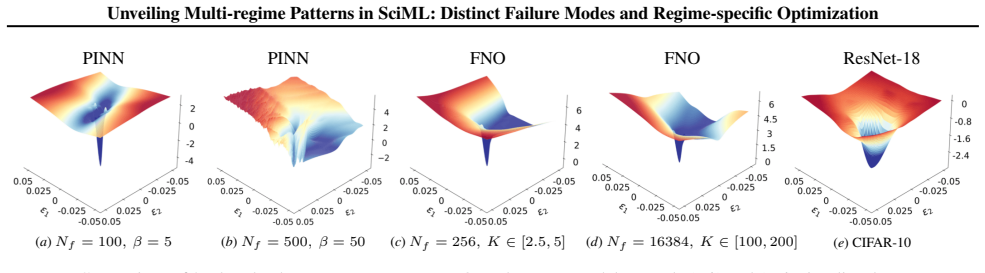
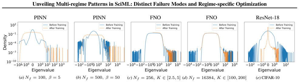
Neural networks trained under different hyperparameter settings can fall into distinct training "regimes," with consistent behavior within regimes and qualitative differences across regimes. In this paper, we study such multi-regime behavior in scientific machine learning (SciML) models through a regime-aware diagnostic framework that jointly analyzes performance, training dynamics, and loss-landscape geometry. We identify three key findings: (i) a consistent three-regime structure emerges across many standard SciML models, different constraint enforcements, and various optimizer designs; (ii) optimization effectiveness is regime-specific, with no single method performing well across all regimes; and (iii) SciML models can exhibit fine-grained failure modes that can challenge conventional interpretations of standard loss-landscape metrics. Our results provide an approach to establish a unified, task-oblivious perspective on failure modes in SciML and to inform regime-aware guidance for improving robustness. We validate these findings across widely-used SciML models, including physics-informed neural networks, neural operators, and neural ordinary differential equations, on benchmarks spanning representative ordinary and partial differential equations.

Editorial analysis

A structured set of objections, weighed in public.

Desk editor's note, referee report, simulated authors' rebuttal, and a circularity audit. Tearing a paper down is the easy half of reading it; the pith above is the substance, this is the friction.

Desk Editor's Note private letter to a colleague

The paper claims a consistent three-regime structure across SciML models but the diagnostic framework's thresholds or clustering choices could be creating that partition rather than revealing it.

read the letter

The main point is that this work identifies three training regimes in SciML that appear across PINNs, neural operators, and neural ODEs, with optimizer performance varying by regime. They back this with a diagnostic that pulls together accuracy, dynamics, and landscape geometry on standard ODE and PDE benchmarks.

What stands out is the breadth of the tests: different constraint enforcements and optimizer families all show the same three-way split. That multi-model, multi-problem check is the concrete contribution if the regimes survive closer inspection. The claim that no single optimizer works everywhere is also useful for people who have tried swapping Adam for L-BFGS and seen mixed results.

The soft spot is the one the stress test flags. The abstract gives no numbers on how the regimes are defined—whether fixed quantiles on gradient variance, Hessian trace, or some unsupervised step—and whether those cutoffs stayed constant across every model family. If the framework re-tunes per experiment or normalizes features in a way that favors three clusters, the “consistent structure” could be an artifact. The fine-grained failure modes section sounds like it might just be restating known issues with loss-landscape metrics rather than overturning them.

This is for readers who already work on SciML robustness and want a practical way to diagnose training problems. It is not yet ready for someone looking for a settled taxonomy.

I would send it to review. The idea is worth testing properly, the validation scope is reasonable, and the authors are not obviously overclaiming in the abstract. A referee can check whether the regime boundaries are stable under small changes to the diagnostic.

Referee Report

2 major / 2 minor

Summary. The paper introduces a regime-aware diagnostic framework that jointly examines performance metrics, training dynamics, and loss-landscape geometry to identify multi-regime behavior in SciML models. It claims that a consistent three-regime structure appears across PINNs, neural operators, and neural ODEs under varied constraint enforcements and optimizers; that no single optimizer works well across all regimes; and that fine-grained failure modes exist that challenge standard loss-landscape interpretations. These findings are validated on representative ODE and PDE benchmarks.

Significance. If the three-regime partition is shown to be intrinsic to the optimization dynamics rather than an artifact of the diagnostic choices, the work could supply a task-oblivious taxonomy of SciML failure modes and motivate regime-aware training protocols. The breadth of models and benchmarks tested is a positive feature; however, the absence of explicit sensitivity checks on the framework's internal parameters limits the strength of the consistency claim.

major comments (2)

[Section 3] Diagnostic framework (Section 3 and associated figures): the central claim of a 'consistent three-regime structure' across model families requires demonstration that the partition is insensitive to the specific feature set, distance metric, normalization, or clustering cutoff employed. The manuscript should include an ablation varying these choices (or reporting the exact fixed thresholds used uniformly) and showing that the number and boundaries of regimes remain stable; without this, the observed structure could be induced by the analysis pipeline rather than the loss surfaces themselves.
[Section 4.2] Regime-specific optimization results (Section 4.2, Tables 2-4): the statement that 'no single method performing well across all regimes' is load-bearing for the practical takeaway, yet the quantitative support (e.g., win rates or relative error distributions per regime) is not accompanied by statistical significance tests across the multiple random seeds or hyperparameter sweeps. The reported performance gaps could be within noise for some regime-optimizer pairs.

minor comments (2)

Notation for the loss-landscape features (e.g., gradient-norm variance, Hessian-trace quantiles) should be defined once in a dedicated table or subsection rather than introduced piecemeal in the text.
Figure captions for the regime visualizations should explicitly state the exact hyperparameter settings and random seeds used to generate each panel so that the consistency claim can be reproduced.

Simulated Author's Rebuttal

2 responses · 0 unresolved

We appreciate the referee's feedback on our manuscript. The comments highlight areas where additional analysis can strengthen our claims regarding the robustness of the regime identification and the statistical support for regime-specific optimization. We outline our responses below and commit to incorporating the suggested revisions.

read point-by-point responses

Referee: [Section 3] Diagnostic framework (Section 3 and associated figures): the central claim of a 'consistent three-regime structure' across model families requires demonstration that the partition is insensitive to the specific feature set, distance metric, normalization, or clustering cutoff employed. The manuscript should include an ablation varying these choices (or reporting the exact fixed thresholds used uniformly) and showing that the number and boundaries of regimes remain stable; without this, the observed structure could be induced by the analysis pipeline rather than the loss surfaces themselves.

Authors: We thank the referee for this important observation. To address this, we will conduct an ablation study in the revised version by varying the feature set, distance metrics, normalization methods, and clustering cutoffs. We will demonstrate that the three-regime structure persists across these variations, thereby strengthening the claim that the partition reflects intrinsic properties of the loss surfaces. Additionally, we will explicitly report the fixed thresholds used in our analysis. revision: yes
Referee: [Section 4.2] Regime-specific optimization results (Section 4.2, Tables 2-4): the statement that 'no single method performing well across all regimes' is load-bearing for the practical takeaway, yet the quantitative support (e.g., win rates or relative error distributions per regime) is not accompanied by statistical significance tests across the multiple random seeds or hyperparameter sweeps. The reported performance gaps could be within noise for some regime-optimizer pairs.

Authors: We agree that statistical validation is necessary to support the claim. In the revision, we will include statistical significance tests (such as paired t-tests or Wilcoxon tests) across the random seeds for the performance differences between optimizers in each regime. This will confirm whether the observed gaps are statistically significant or within noise levels. revision: yes

Circularity Check

0 steps flagged

No detectable circularity; regime identification presented as empirical observation without reduction to fitted inputs or self-citations

full rationale

The abstract and provided context describe an empirical diagnostic framework applied across multiple SciML models to identify a three-regime structure, with claims resting on observed consistency in performance, dynamics, and geometry rather than any self-definitional loop, fitted parameter renamed as prediction, or load-bearing self-citation. No equations, ansatzes, or uniqueness theorems are quoted that would make the regime partition equivalent to the analysis choices by construction. The framework is presented as task-oblivious and validated on standard benchmarks, keeping the derivation self-contained against external data.

Axiom & Free-Parameter Ledger

0 free parameters · 0 axioms · 0 invented entities

Based on the abstract, no free parameters, axioms, or invented entities are specified.

pith-pipeline@v0.9.1-grok · 5759 in / 885 out tokens · 27797 ms · 2026-06-29T13:14:35.873390+00:00 · methodology

discussion (0)

Reference graph

Works this paper leans on

4 extracted references · 1 canonical work pages · 1 internal anchor

[1]

write newline

" write newline "" before.all 'output.state := FUNCTION n.dashify 't := "" t empty not t #1 #1 substring "-" = t #1 #2 substring "--" = not "--" * t #2 global.max substring 't := t #1 #1 substring "-" = "-" * t #2 global.max substring 't := while if t #1 #1 substring * t #2 global.max substring 't := if while FUNCTION format.date year duplicate empty "emp...
[2]

@esa (Ref

\@ifxundefined[1] #1\@undefined \@firstoftwo \@secondoftwo \@ifnum[1] #1 \@firstoftwo \@secondoftwo \@ifx[1] #1 \@firstoftwo \@secondoftwo [2] @ #1 \@temptokena #2 #1 @ \@temptokena \@ifclassloaded agu2001 natbib The agu2001 class already includes natbib coding, so you should not add it explicitly Type <Return> for now, but then later remove the command n...
[3]

\@lbibitem[] @bibitem@first@sw\@secondoftwo \@lbibitem[#1]#2 \@extra@b@citeb \@ifundefined br@#2\@extra@b@citeb \@namedef br@#2 \@nameuse br@#2\@extra@b@citeb \@ifundefined b@#2\@extra@b@citeb @num @parse #2 @tmp #1 NAT@b@open@#2 NAT@b@shut@#2 \@ifnum @merge>\@ne @bibitem@first@sw \@firstoftwo \@ifundefined NAT@b*@#2 \@firstoftwo @num @NAT@ctr \@secondoft...
[4]

Rethinking generalization requires revisiting old ideas: statistical mechanics approaches and complex learning behavior

@open @close @open @close and [1] URL: #1 \@ifundefined chapter * \@mkboth \@ifxundefined @sectionbib * \@mkboth * \@mkboth\@gobbletwo \@ifclassloaded amsart * \@ifclassloaded amsbook * \@ifxundefined @heading @heading NAT@ctr thebibliography [1] @ \@biblabel @NAT@ctr \@bibsetup #1 @NAT@ctr @ @openbib .11em \@plus.33em \@minus.07em 4000 4000 `\.\@m @bibit...

work page internal anchor Pith review Pith/arXiv arXiv doi:10.48550/arxiv.1710.09553 2019

[1] [1]

write newline

" write newline "" before.all 'output.state := FUNCTION n.dashify 't := "" t empty not t #1 #1 substring "-" = t #1 #2 substring "--" = not "--" * t #2 global.max substring 't := t #1 #1 substring "-" = "-" * t #2 global.max substring 't := while if t #1 #1 substring * t #2 global.max substring 't := if while FUNCTION format.date year duplicate empty "emp...

[2] [2]

@esa (Ref

\@ifxundefined[1] #1\@undefined \@firstoftwo \@secondoftwo \@ifnum[1] #1 \@firstoftwo \@secondoftwo \@ifx[1] #1 \@firstoftwo \@secondoftwo [2] @ #1 \@temptokena #2 #1 @ \@temptokena \@ifclassloaded agu2001 natbib The agu2001 class already includes natbib coding, so you should not add it explicitly Type <Return> for now, but then later remove the command n...

[3] [3]

\@lbibitem[] @bibitem@first@sw\@secondoftwo \@lbibitem[#1]#2 \@extra@b@citeb \@ifundefined br@#2\@extra@b@citeb \@namedef br@#2 \@nameuse br@#2\@extra@b@citeb \@ifundefined b@#2\@extra@b@citeb @num @parse #2 @tmp #1 NAT@b@open@#2 NAT@b@shut@#2 \@ifnum @merge>\@ne @bibitem@first@sw \@firstoftwo \@ifundefined NAT@b*@#2 \@firstoftwo @num @NAT@ctr \@secondoft...

[4] [4]

Rethinking generalization requires revisiting old ideas: statistical mechanics approaches and complex learning behavior

@open @close @open @close and [1] URL: #1 \@ifundefined chapter * \@mkboth \@ifxundefined @sectionbib * \@mkboth * \@mkboth\@gobbletwo \@ifclassloaded amsart * \@ifclassloaded amsbook * \@ifxundefined @heading @heading NAT@ctr thebibliography [1] @ \@biblabel @NAT@ctr \@bibsetup #1 @NAT@ctr @ @openbib .11em \@plus.33em \@minus.07em 4000 4000 `\.\@m @bibit...

work page internal anchor Pith review Pith/arXiv arXiv doi:10.48550/arxiv.1710.09553 2019