Inverse generalised spin models of answers to questionnaires
Pith reviewed 2026-06-28 23:44 UTC · model grok-4.3
The pith
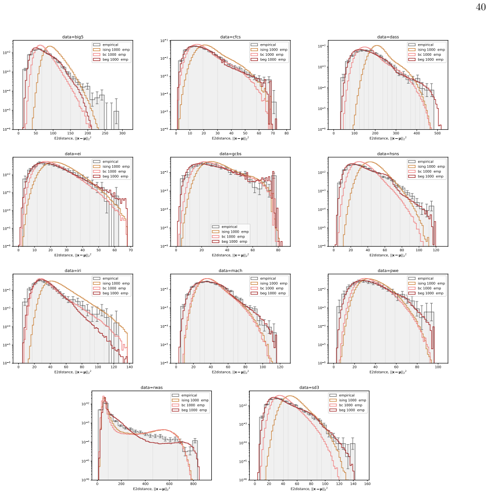
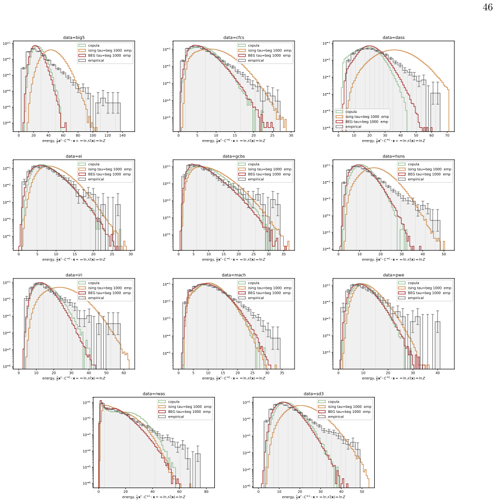
The BEG model captures the distribution of distances to the mean in ordinal questionnaire responses better than Ising, Blume-Capel or Gaussian models.
A machine-rendered reading of the paper's core claim, the machinery that carries it, and where it could break.
Core claim
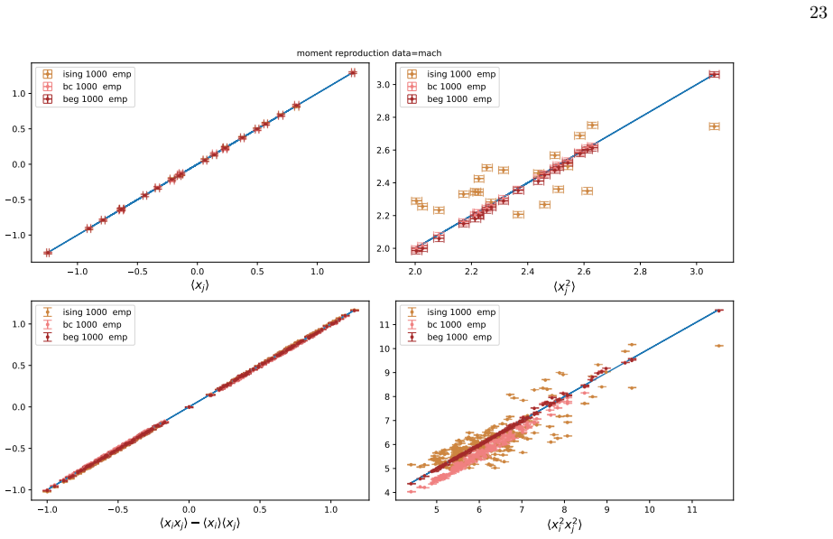
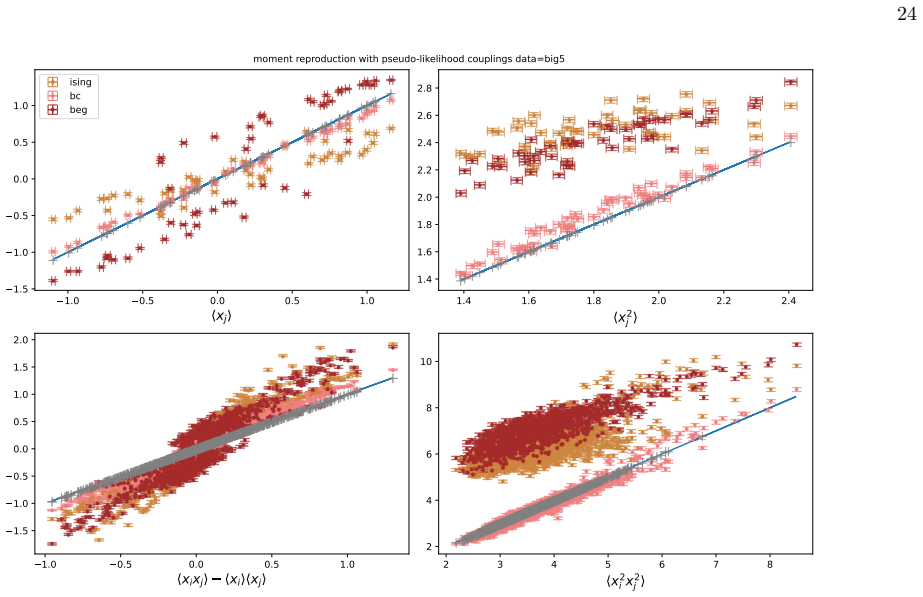
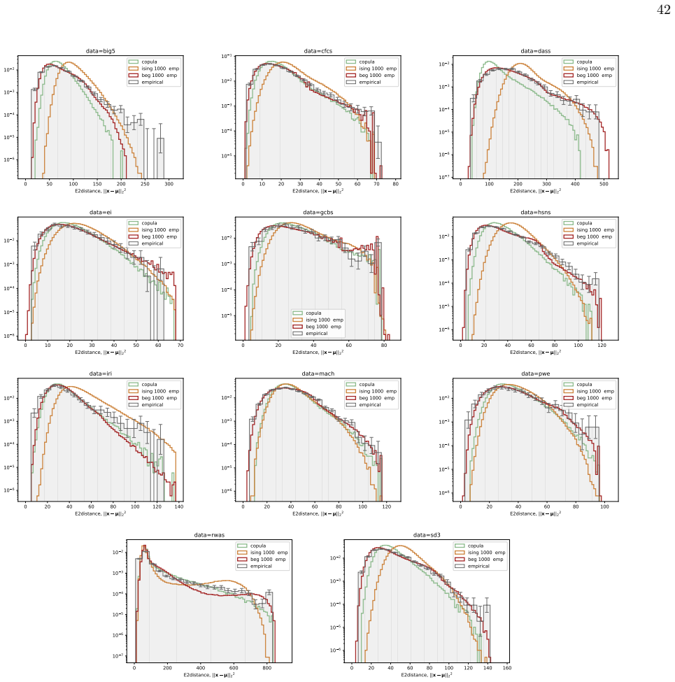
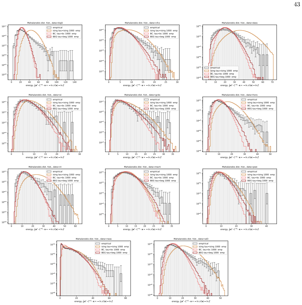
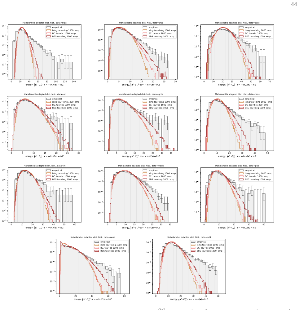
We infer and analyse three generalised spin models of ordinal questionnaire data: the generalised Ising, Blume-Capel (BC), and Blume-Emery-Griffiths (BEG) models. We prove the concavity of the maximum likelihood estimation of the parameters, as well as the gauge invariance of the Ising and BC models. Afterwards, we propose an inference protocol of approximated likelihood maximisation, based on the Monte Carlo estimation of the likelihood gradients. We apply this procedure to eleven psychometric and sociological questionnaires, comparing the inferred spin models against the multivariate Gaussian. The BEG model systematically outperforms the other models in capturing the distribution of distan
What carries the argument
Monte Carlo approximated likelihood maximisation applied to the energy functions of the generalised Ising, Blume-Capel and Blume-Emery-Griffiths models on ordinal response vectors.
If this is right
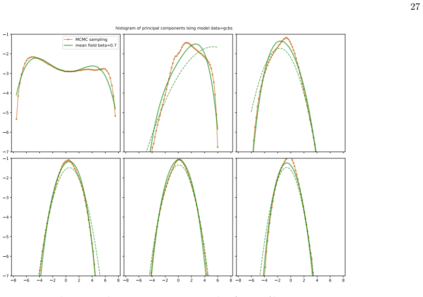
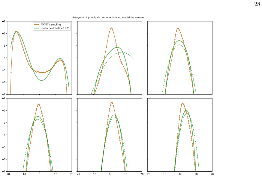
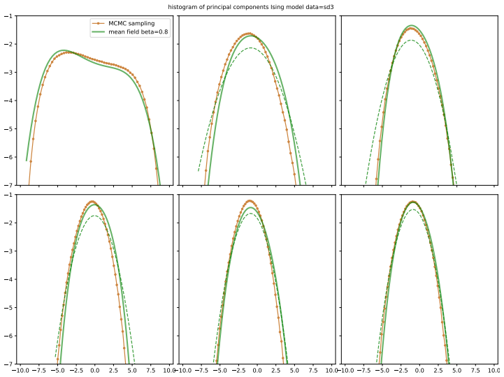
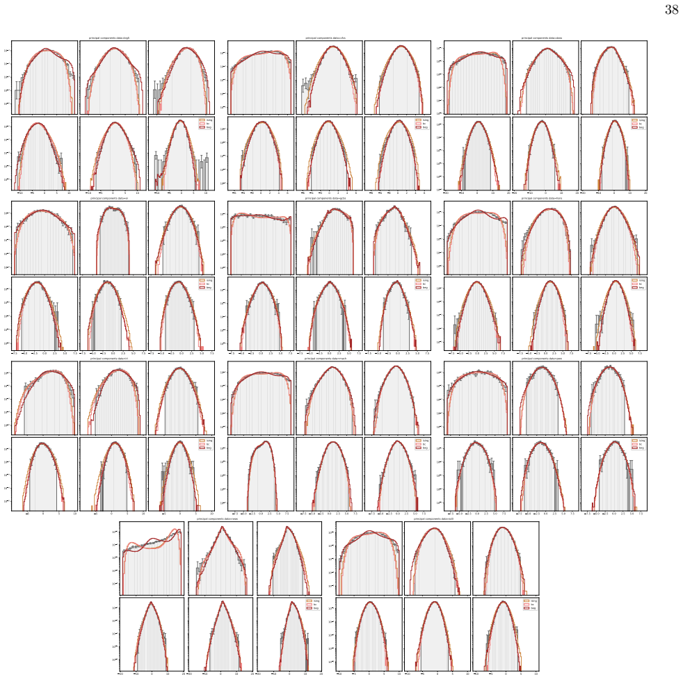
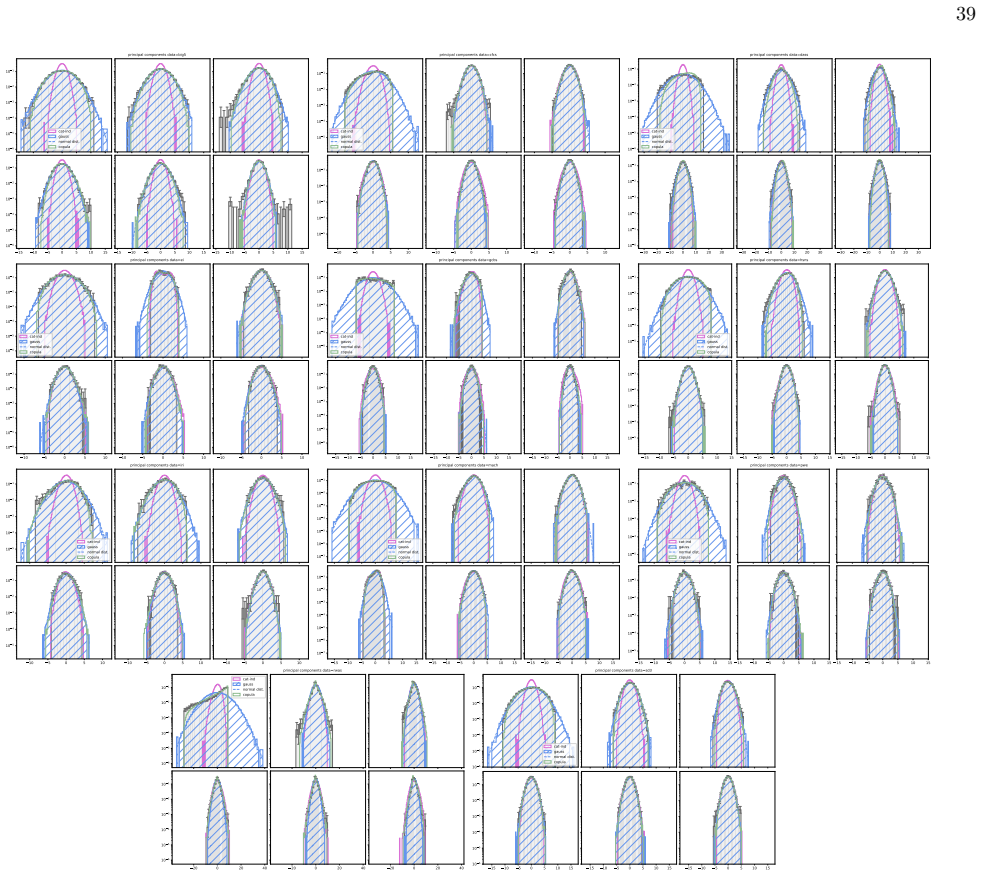
- Multi-modality in principal-component histograms of questionnaire data corresponds to coexistence of stable and metastable phases in the spin models under mean-field theory.
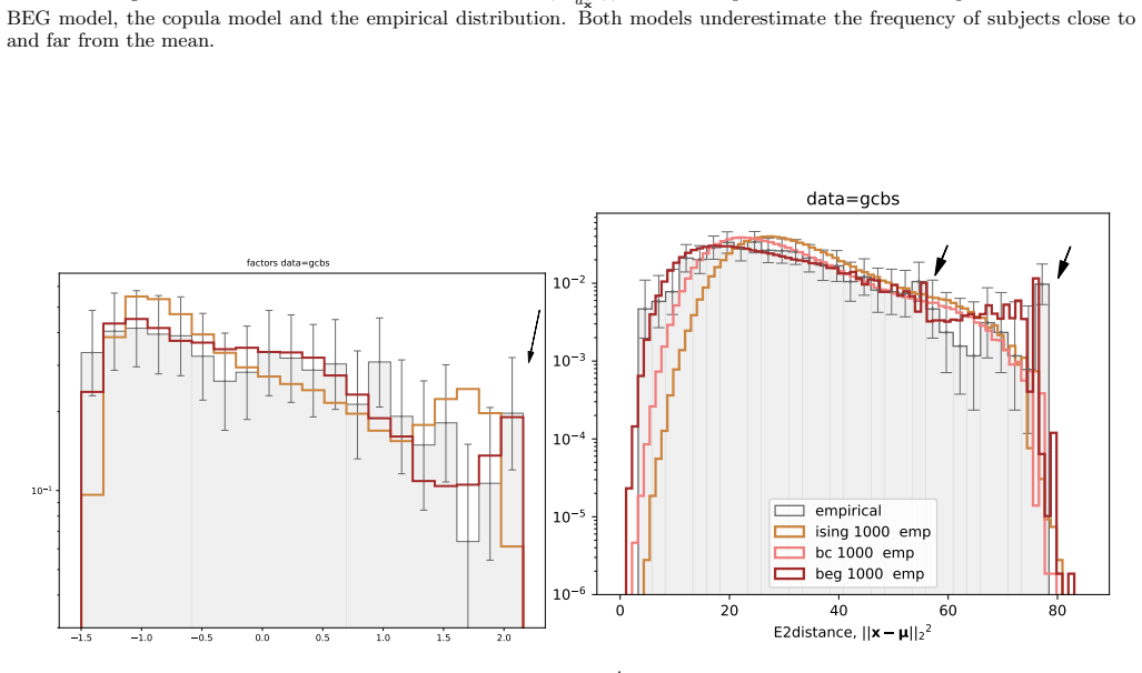
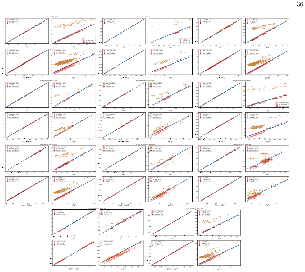
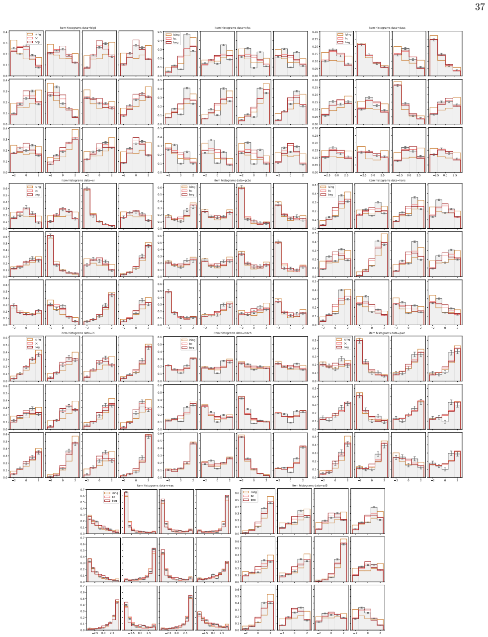
- The abundance of both outliers and mean responders in real questionnaires is reproduced by the pair and higher-order interaction terms present in the BEG energy function.
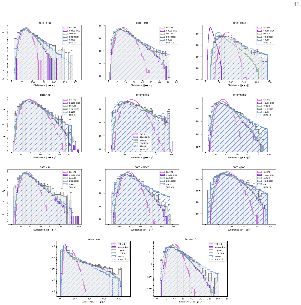
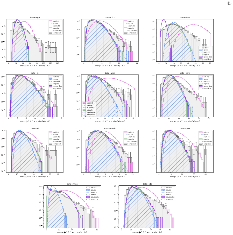
- Gaussian models miss the non-linear polarisation structure that the spin models partially recover.
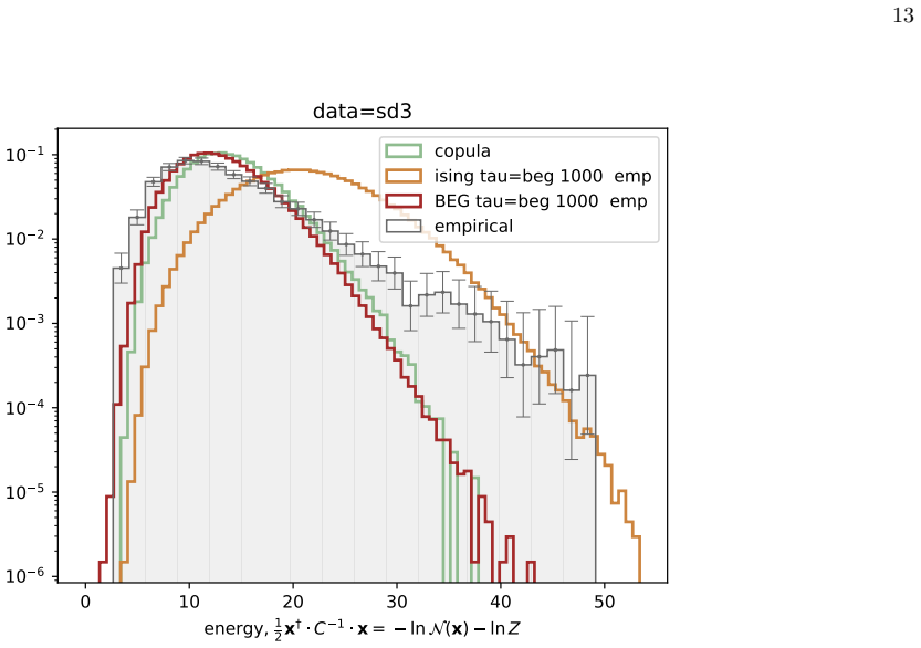
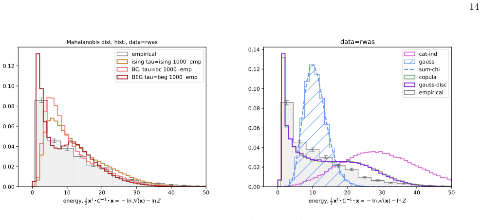
- All three spin models and the Gaussian underestimate the frequency of extreme Mahalanobis distances, indicating residual heavy-tailed structure not captured by any of them.
Where Pith is reading between the lines
- If the BEG model continues to outperform on new datasets, questionnaire-based psychological constructs could be re-analysed as phase-coexistence phenomena rather than linear factor structures.
- The failure to capture Mahalanobis tails suggests that future model extensions should incorporate explicit outlier-generating mechanisms or long-range couplings beyond the current energy functions.
- The gauge invariance proved for the Ising and BC models implies that only relative differences in response patterns are identifiable, which may limit absolute-scale interpretations of fitted parameters.
Load-bearing premise
Ordinal questionnaire responses are adequately described by the energy functions of the generalised Ising, Blume-Capel and Blume-Emery-Griffiths models.
What would settle it
Generate synthetic response vectors from the fitted BEG model on a held-out questionnaire and check whether the histogram of Mahalanobis distances to the mean matches the empirical histogram within sampling error; persistent underestimation of the heavy tail would falsify the claim of superior predictive power.
Figures
read the original abstract
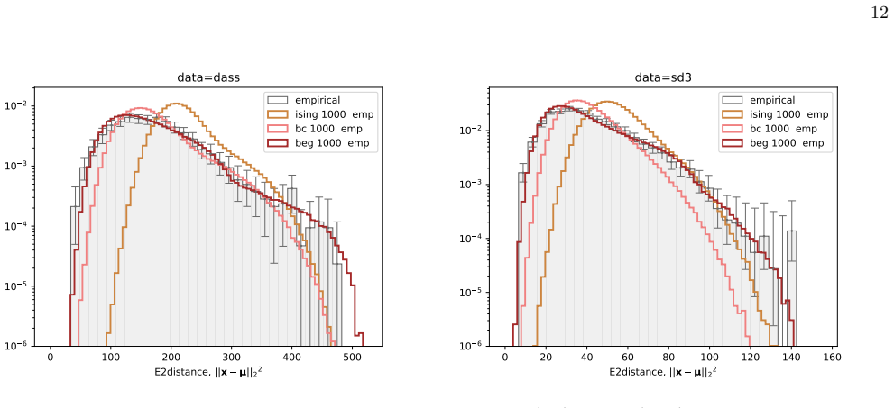
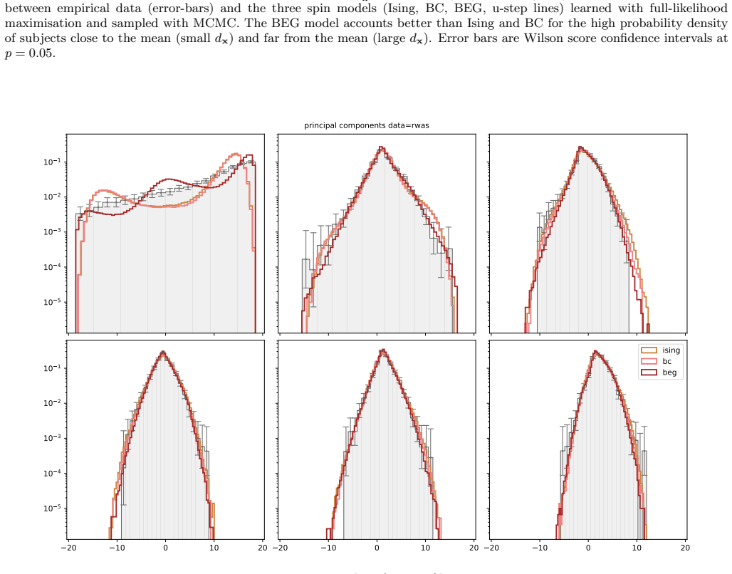
Network psychometrics conceptualises psychological constructs as emergent properties of systems of interacting variables. Energy-based probabilistic models have gained popularity as models of these interactions, but their psychometric application has so far been limited, since most implementations assume binary or ternary responses and rely on limiting inference assumptions. We infer and analyse three generalised spin models of ordinal questionnaire data: the generalised Ising, Blume-Capel (BC), and Blume-Emery-Griffiths (BEG) models. We prove the concavity of the maximum likelihood estimation of the parameters, as well as the gauge invariance of the Ising and BC models. Afterwards, we propose an inference protocol of approximated likelihood maximisation, based on the Monte Carlo estimation of the likelihood gradients. We apply this procedure to eleven psychometric and sociological questionnaires, comparing the inferred spin models against the multivariate Gaussian. We then assess whether the inferred models reproduce the empirical features of the data in terms of principal-component histograms, and histograms of Euclidean and Mahalanobis distances to the mean answer. The multi-modality observed in the histograms of principal components is partially captured by the spin models. This trait of polarisation can be understood, in the light of mean-field theory, as coexistence of stable and metastable phases of the spin models. The BEG model systematically outperforms the other models in capturing the distribution of distances to the mean, while all models underestimate the heavy tails of the Mahalanobis distance. Overall, the analysis witnesses the predictive power of the BEG model, able to account better than others for the abundance of outliers and mean responders, and reveals highly non-linear features of questionnaire data that both Gaussian and spin models fail to account for.
Editorial analysis
A structured set of objections, weighed in public.
Referee Report
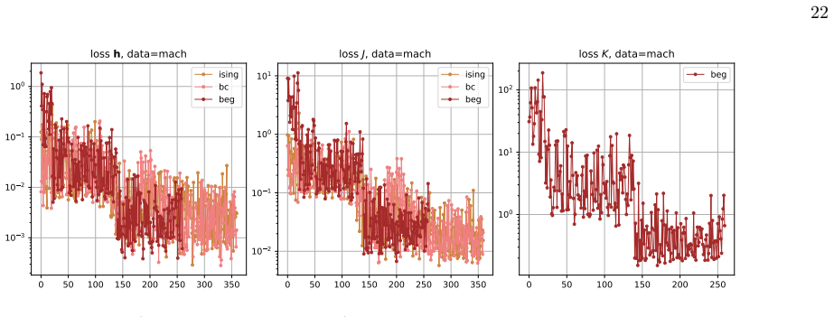
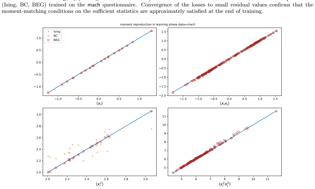
Summary. The paper introduces three generalised spin models (Ising, Blume-Capel, BEG) for ordinal questionnaire responses, proves concavity of exact MLE and gauge invariance for Ising/BC, proposes an MC-based approximated likelihood maximisation protocol, fits the models plus a multivariate Gaussian to eleven datasets, and evaluates reproduction of empirical PC histograms and Euclidean/Mahalanobis distance-to-mean histograms. It concludes that the models partially capture multi-modality (interpretable via mean-field phase coexistence) and that BEG systematically outperforms the others on distance distributions while all underestimate Mahalanobis heavy tails.
Significance. If the central performance claims hold after addressing inference diagnostics, the work would usefully extend energy-based models beyond binary/ternary cases in network psychometrics, providing concrete evidence that BEG can better account for outliers and mean-responders than Gaussian baselines on real data. The explicit proofs of concavity and gauge invariance, together with the multi-dataset application, constitute reusable technical contributions even if the histogram comparisons remain qualitative.
major comments (2)
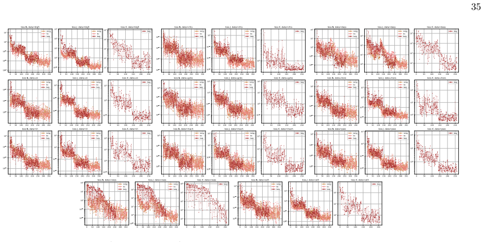
- [Abstract (inference protocol) and results on distance histograms] The claim that BEG systematically outperforms Ising/BC/Gaussian on distance-to-mean histograms rests on parameters obtained via Monte Carlo gradient estimates for MLE. The manuscript proves concavity only for the exact log-likelihood; no diagnostics (chain length, autocorrelation, effective sample size, or bias/variance quantification of the MC gradient) are reported for the eleven datasets. Because the Gaussian has closed-form MLE while the spin models use the approximation, any observed outperformance could be an artifact of optimisation error rather than model structure. This directly affects the central predictive-power conclusion.
- [Abstract (assessment of inferred models) and empirical feature comparisons] Performance assessment relies on visual/qualitative comparison of histograms without reported quantitative metrics (e.g., Kolmogorov-Smirnov statistics, Wasserstein distances, or bootstrap error bars), details on data exclusion criteria, or robustness checks. The abstract states that multi-modality is 'partially captured' and BEG 'systematically outperforms,' but the absence of these measures prevents judging whether the differences are statistically meaningful or sensitive to fitting choices.
minor comments (2)
- [Model definitions] Notation for the energy functions and the precise mapping from ordinal responses to spin states should be stated explicitly with an equation or table early in the methods, to allow readers to verify the generalisation from binary Ising to the BEG case.
- [Inference protocol] The manuscript should clarify whether the same MC protocol (number of samples, burn-in, etc.) was used uniformly across all eleven questionnaires or tuned per dataset, as this affects reproducibility of the reported parameters.
Simulated Author's Rebuttal
We thank the referee for the constructive and detailed comments. We address each major point below and will revise the manuscript to incorporate the suggested improvements.
read point-by-point responses
-
Referee: [Abstract (inference protocol) and results on distance histograms] The claim that BEG systematically outperforms Ising/BC/Gaussian on distance-to-mean histograms rests on parameters obtained via Monte Carlo gradient estimates for MLE. The manuscript proves concavity only for the exact log-likelihood; no diagnostics (chain length, autocorrelation, effective sample size, or bias/variance quantification of the MC gradient) are reported for the eleven datasets. Because the Gaussian has closed-form MLE while the spin models use the approximation, any observed outperformance could be an artifact of optimisation error rather than model structure. This directly affects the central predictive-power conclusion.
Authors: We agree that the lack of reported diagnostics for the Monte Carlo gradient estimates represents a gap that weakens confidence in the performance comparisons. Although the concavity result holds for the exact likelihood, the practical MLEs rely on the approximation, and the closed-form Gaussian MLE creates an asymmetry. In the revision we will add, for each of the eleven datasets, the Monte Carlo chain lengths employed, autocorrelation times, effective sample sizes, and quantitative estimates of bias and variance in the gradient estimates. These diagnostics will allow readers to evaluate whether the observed BEG advantage is attributable to model structure rather than optimisation error. revision: yes
-
Referee: [Abstract (assessment of inferred models) and empirical feature comparisons] Performance assessment relies on visual/qualitative comparison of histograms without reported quantitative metrics (e.g., Kolmogorov-Smirnov statistics, Wasserstein distances, or bootstrap error bars), details on data exclusion criteria, or robustness checks. The abstract states that multi-modality is 'partially captured' and BEG 'systematically outperforms,' but the absence of these measures prevents judging whether the differences are statistically meaningful or sensitive to fitting choices.
Authors: We concur that quantitative metrics and robustness information are necessary to substantiate the abstract claims. We will revise the manuscript to include Kolmogorov-Smirnov statistics and Wasserstein distances comparing the empirical and model-generated histograms for both principal-component and distance-to-mean distributions, together with bootstrap-derived error bars. We will also document the precise data-exclusion criteria applied to the eleven questionnaires and report results of robustness checks obtained by varying Monte Carlo sample size and optimisation initial conditions. These additions will permit a statistically grounded assessment of the partial capture of multi-modality and the relative performance of the models. revision: yes
Circularity Check
No circularity: standard MLE fitting followed by independent statistic checks
full rationale
The paper performs approximated MLE on the full joint distribution of questionnaire responses, then evaluates reproduction of derived histograms (PC, Euclidean/Mahalanobis distances). These checks are not the optimized objective itself and are not equivalent to the inputs by construction. No self-definitional steps, no fitted quantities renamed as predictions, and no load-bearing self-citations or imported uniqueness theorems appear in the derivation. The comparison to the closed-form Gaussian baseline provides an external reference point. This is ordinary in-sample model assessment, not a reduction of the claimed result to its own fitted values.
Axiom & Free-Parameter Ledger
free parameters (1)
- spin couplings and fields
axioms (1)
- domain assumption Ordinal responses can be represented as discrete spin states whose joint distribution is given by an energy function of the generalized Ising/BC/BEG form.
Reference graph
Works this paper leans on
-
[1]
J. Kruis, G. Maris, M. Marsman, M. Bolsinova, and H. L. J. van der Maas, Scientific Reports10, 10.1038/s41598-020- 73181-2 (2020)
-
[2]
Lunansky, G
G. Lunansky, G. A. Bonanno, T. F. Blanken, C. D. van Borkulo, A. O. J. Cramer, and D. Borsboom, Psychological Review 132, 1396–1409 (2025)
2025
-
[3]
Hoffman, D
M. Hoffman, D. Steinley, T. J. Trull, and K. J. Sher, Clinical Psychological Science6, 506–516 (2017)
2017
-
[4]
A. Finnemann, D. Borsboom, L. Waldorp, M. Marsman, and H. L. J. van der Maas 10.31219/osf.io/yc3p7 v2 (2026). 17
-
[5]
Rabe and K
S. Rabe and K. V. Mardia, Journal of Applied Statistics21, 479–494 (1994)
1994
-
[6]
L. Waldorp, T. Pham, and H. L. J. van der Maas, The European Physical Journal B98, 10.1140/epjb/s10051-025-01060-8 (2025)
-
[7]
Blume, Physical Review141, 517–524 (1966)
M. Blume, Physical Review141, 517–524 (1966)
1966
-
[8]
Capel, Physica32, 966 (1966)
H. Capel, Physica32, 966 (1966)
1966
-
[9]
Waldorp, J
L. Waldorp, J. Dalege, M. Marsman, A. Finnemann, I. Ferri, and H. L. van der Maas, Physica A: Statistical Mechanics and its Applications , 131554 (2026)
2026
-
[10]
Blume, V
M. Blume, V. J. Emery, and R. B. Griffiths, Physical Review A4, 1071–1077 (1971)
1971
- [11]
-
[12]
J.-P. Stein, T. Messingschlager, T. Gnambs, F. Hutmacher, and M. Appel, Scientific Reports14, 10.1038/s41598-024- 53335-2 (2024)
-
[13]
Moessner and A
R. Moessner and A. P. Ramirez, Physics Today59, 24–29 (2006)
2006
-
[14]
Ising, Zeitschrift f¨ ur Physik31, 253 (1925)
E. Ising, Zeitschrift f¨ ur Physik31, 253 (1925)
1925
-
[15]
Onsager, Physical review65, 117 (1944)
L. Onsager, Physical review65, 117 (1944)
1944
-
[16]
R. J. Baxter, inIntegrable systems in statistical mechanics(World Scientific, 1985) pp. 5–63
1985
-
[17]
Mussardo,Statistical field theory: an introduction to exactly solved models in statistical physics(Oxford University Press, 2010)
G. Mussardo,Statistical field theory: an introduction to exactly solved models in statistical physics(Oxford University Press, 2010)
2010
-
[18]
Pathria and P
R. Pathria and P. Beale, New York (2011)
2011
-
[19]
Krinsky and D
S. Krinsky and D. Mukamel, Phys. Rev. B12, 211 (1975)
1975
-
[20]
W. J. Camp, D. Saul, J. Van Dyke, and M. Wortis, Physical Review B14, 3990 (1976)
1976
-
[21]
A. N. Berker and M. Wortis, Physical Review B14, 4946 (1976)
1976
-
[22]
I. D. Lawrie, S. Sarbach,et al., Phase transitions and critical phenomena9(1984)
1984
-
[23]
E. T. Jaynes, Phys. Rev.106, 620 (1957)
1957
-
[24]
E. T. Jaynes, Phys. Rev.108, 171 (1957)
1957
-
[25]
H. C. Nguyen, R. Zecchina, and J. Berg, Advances in Physics66, 197 (2017), https://doi.org/10.1080/00018732.2017.1341604
-
[26]
Besag, Journal of the Royal Statistical Society: Series D (The Statistician)24, 179 (1975)
J. Besag, Journal of the Royal Statistical Society: Series D (The Statistician)24, 179 (1975)
1975
-
[27]
Aurell and M
E. Aurell and M. Ekeberg, Physical review letters108, 090201 (2012)
2012
-
[28]
Ekeberg, C
M. Ekeberg, C. L¨ ovkvist, Y. Lan, M. Weigt, and E. Aurell, Physical Review E—Statistical, Nonlinear, and Soft Matter Physics87, 012707 (2013)
2013
-
[29]
Ekeberg, T
M. Ekeberg, T. Hartonen, and E. Aurell, Journal of Computational Physics276, 341 (2014)
2014
-
[30]
Decelle and F
A. Decelle and F. Ricci-Tersenghi, Physical review letters112, 070603 (2014)
2014
-
[31]
Cocco, C
S. Cocco, C. Feinauer, M. Figliuzzi, R. Monasson, and M. Weigt, Reports on Progress in Physics81, 032601 (2018)
2018
-
[32]
Ravikumar, M
P. Ravikumar, M. J. Wainwright, and J. D. Lafferty, The Annals of Statistics38, 1287 (2010)
2010
-
[33]
D. C. Liu and J. Nocedal, Mathematical programming45, 503 (1989)
1989
-
[34]
Nocedal and S
J. Nocedal and S. Wright, New York (2006)
2006
-
[35]
scipy.optimize.minimiz-lbfgsb,https://docs.scipy.org/doc/scipy/reference/optimize.minimize-lbfgsb.html, ac- cessed: 2026-04
2026
-
[36]
G. E. Hinton, Neural computation14, 1771 (2002)
2002
-
[37]
Tieleman, inProceedings of the 25th international conference on Machine learning(2008) pp
T. Tieleman, inProceedings of the 25th international conference on Machine learning(2008) pp. 1064–1071
2008
-
[38]
G. E. Hinton, inNeural Networks: Tricks of the Trade: Second Edition(Springer, 2012) pp. 599–619
2012
-
[39]
Decelle and F
A. Decelle and F. Ricci-Tersenghi, Physical Review E94, 012112 (2016)
2016
-
[40]
M. J. Wainwright and M. I. Jordan, Foundations and Trends®in Machine Learning1, 1 (2008)
2008
-
[41]
D. J. MacKay,Information theory, inference and learning algorithms(Cambridge university press, 2003)
2003
-
[42]
D. P. Kingma and J. Ba, Adam: A method for stochastic optimization (2017), arXiv:1412.6980 [cs.LG]
work page internal anchor Pith review Pith/arXiv arXiv 2017
-
[43]
Pelissetto, Summer School in Theoretical Physics and Bonini, M
A. Pelissetto, Summer School in Theoretical Physics and Bonini, M. and Marchesini, G. and Onofri, E. (1993)
1993
-
[44]
Sokal, Functional integration: Basics and applications (Springer US, Boston, MA, 1997) Chap
A. Sokal, Functional integration: Basics and applications (Springer US, Boston, MA, 1997) Chap. Monte Carlo Methods in Statistical Mechanics: Foundations and New Algorithms, pp. 131–192
1997
-
[45]
Binder, Reports on Progress in Physics60, 487 (1997)
K. Binder, Reports on Progress in Physics60, 487 (1997)
1997
-
[46]
Open-source psychometrics project,https://openpsychometrics.org/_rawdata/
-
[47]
Albiero, S
P. Albiero, S. Ingoglia, A. Lo Coco,et al., Testing Psicometria Metodologia13, 107 (2006)
2006
-
[48]
P. J. Jordan, N. M. Ashkanasy, and C. E. Hartel, Academy of Management review27, 361 (2002)
2002
-
[49]
D. D. Vachon and D. R. Lynam, Assessment23, 135 (2016)
2016
-
[50]
Iba˜ nez-Berganza and A
M. Iba˜ nez-Berganza and A. Armanetti, qspin: Generalized ising / blume–capel / blume–emery–griffiths inference for ordinal questionnaire data (2026)
2026
-
[51]
Furnham, Personality and individual differences7, 385 (1986)
A. Furnham, Personality and individual differences7, 385 (1986)
1986
-
[52]
Ib´ a˜ nez Berganza, C
M. Ib´ a˜ nez Berganza, C. Lucibello, F. Santucci, T. Gili, and A. Gabrielli, Phys. Rev. E108, 024313 (2023)
2023
-
[53]
Finnemann, D
A. Finnemann, D. Borsboom, S. Epskamp, and H. L. van der Maas, Psych3, 593 (2021)
2021
-
[54]
M´ ezard, G
M. M´ ezard, G. Parisi, M. A. Virasoro, and D. J. Thouless, Spin glass theory and beyond (1988)
1988
-
[55]
A. J. Bray and M. A. Moore, Journal of Physics C: Solid State Physics13, L469 (1980)
1980
-
[56]
Y. V. Fyodorov, Physical review letters92, 240601 (2004)
2004
-
[57]
de Mulatier and M
C. de Mulatier and M. Marsili, Phys. Rev. E111, 054307 (2025)
2025
-
[58]
D. J. Amit and V. Martin-Mayor,Field theory, the renormalization group, and critical phenomena(McGraw-Hill Interna- 18 tional Book Co., 2005)
2005
-
[59]
P. M. Chaikin, T. C. Lubensky, and T. A. Witten,Principles of condensed matter physics, Vol. 10 (Cambridge university press Cambridge, 1995)
1995
-
[60]
Gil-Pelaez, Biometrika38, 481 (1951)
J. Gil-Pelaez, Biometrika38, 481 (1951)
1951
-
[61]
E. B. Wilson, Journal of the American Statistical Association22, 209 (1927). Appendix A: Pseudo-likelihood maximisation: explicit form The pseudo-likelihood is given by the product over the items of the conditional log-probability of each itemigiven all other items. Fixingx \i, the Hamiltonian of a generalised spin model reduces to a function ofx i alone,...
1927
-
[62]
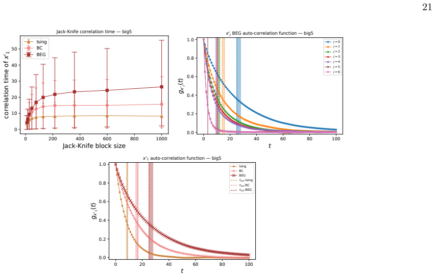
lies in the interval [24.3,28.9] at p= 0.05 (assuming aχ 2 distribution), which is at least 10 4 times smaller than the total number of MCMC sweepsT= 10 7 used for sampling; see Sec. C. time, but about a correlation time for each observableoof interest. When sampling fromTMCMC sweeps, the standard deviation of the average ofoover theTsamples decreases, wh...
-
[63]
(F10), and definingz:=µ−µ 0, the deviations with respect to the minimum-free energy value µ0 in Eq
Zero fields: continuous symmetry-breaking transition In the weak coupling approximation toO(a 2), the solution of the mean field equations (F3) isa 0 =B −1µ0, with µ0 = (βB2)−11M −J −1 ·h.(F13) Substituting in Eq. (F10), and definingz:=µ−µ 0, the deviations with respect to the minimum-free energy value µ0 in Eq. (F13), we get: F=F 0 + 1 2 z† · ˜J·z− 1 24β...
-
[64]
If we now rotate matrixχin the basis ofJeigenvectors, we obtain χ′ km =∂µ ′ k/∂h′ m =δ km(B2β)/(1−(B 2βϵk)), which is regular forβ < β ∗, and diverges atβ ∗ = (B 2ϵ1)−1
Put it differently, using the above relation µj =B 2aj +O(a 2 j), and the mean field self-consistency equations (F3), we haveµ= (B2β)−11M −J −1 ·h+O(a 3), from which we learn that the susceptibility matrixχ ij =∂µ i/∂hj takes the form: 26 χ= (B2β)−11M −J −1 ,(F16) where 1M is the identity matrix inMdimensions. If we now rotate matrixχin the basis ofJeigen...
-
[65]
The free energy in Eq
Non-zero fields and weak disorder: discontinuous onset of a metastable solution We will now adopt theweak disorder approximation, according to which the second eigenvalue ofJis much lower than the first,ϵ 1 ≫ϵ 2. The free energy in Eq. (F10) as a function of the (non-centred) principal components µ′ j :=u † j ·µreads: F=F 0 −h ′ ·µ ′ + 1 2 MX k=1 Ak(β)µ′ ...
-
[66]
The effective free energy ˜F1 develops two local maxima whenever the discriminant of the cubic equation d ˜F1(z)/dz= 0 becomes negative
=−lnR−h ′ 1µ′ 1 + 1 2 A1(β)µ′ 1 2 + G1(β) 24 µ′ 1 4 (F19) whereG k(β) :=−(B 42/B4 2)β−1PM j=1 u4 kj. The effective free energy ˜F1 develops two local maxima whenever the discriminant of the cubic equation d ˜F1(z)/dz= 0 becomes negative. This arises whenever: A1(β)≤ − 27 8 G1(β)h ′ 1 2 1/3 .(F20) For sufficiently lowh ′ 1, there exists a critical value of...
-
[67]
This is shown in Figs
presents two maxima, i.e.β k > β ′ only fork= 1. This is shown in Figs. 11,12 for thegcbs,rwasdatasets. In these figures, we show lnh x′ k for the Ising model versus − ˜Fk +c k, wherec k is an offset minimising the mean squared error with the Ising histogram in the given histogram points. The chosen values ofβ ′ <1 are indicated in the legend. We also sho...
-
[68]
Gauge transformations and gauge invariance Given a shift vectora∈R M, letX ′ =X+adenote the translated state space. We say that the pairξ= (a, f) defines agauge transformationfromM ′ (onX ′) toM(onX) iff: Θ ′ →Θ is invertible and PX+a(x+a|θ ′) =P X(x|f(θ ′))∀x∈X, θ ′ ∈Θ ′.(G1) Since bothfand the translationx7→x+aare invertible, ifξ= (a, f) is a gauge tran...
-
[69]
For a maximum-entropy model with HamiltonianH M(x|θ) = P µ θµCµ(x), two parameter vectors give the same distribution if and only ifH(x|θ)− H(x|θ ′) =cis constant over all statesx∈X
Identifiability A statistical model isidentifiableifθ̸=θ ′ impliesP M(·|θ)̸=P M(·|θ′). For a maximum-entropy model with HamiltonianH M(x|θ) = P µ θµCµ(x), two parameter vectors give the same distribution if and only ifH(x|θ)− H(x|θ ′) =cis constant over all statesx∈X. Since in this case the Hamiltonian is linear inθ, this is equal to H(x|θ−θ ′) =c, so ide...
-
[70]
Strict concavity of the log-likelihood As shown in [78, pp. 62–63], a maximum-entropy model is identifiable in the sense of the definition in subsection G 2 if and only if the Hessian of the log-likelihood is negative definite for all states and parameters (the term that is used in [78, pp. 40,62–63] for an identifiable model is amodel having a minimal re...
-
[71]
Assessment of gauge invariance for the Ising, the BC and the BEG models Keeping in mind the reduction to the case ofN= 1 subjects in the previous subsections, in this and in the next subsection we will just consider the case of one subject. The key ingredient is the binomial identity: (z+c) l =z l + (lower-degree terms inz), so the leading monomial in eac...
-
[72]
Assessment of identifiability for the Ising, the BC and the BEG models The strategy is the same in all three cases. By gauge invariance (§G 1) and invariance of identifiability under gauge transformations (where we use the restricted type of gauge invariance with a uniformain the case of the extended BEG model, as will be seen) we may assume 0∈S, so that ...
discussion (0)
Sign in with ORCID, Apple, or X to comment. Anyone can read and Pith papers without signing in.