SRT: Super-Resolution for Time Series via Disentangled Rectified Flow
Pith reviewed 2026-06-28 23:24 UTC · model grok-4.3
The pith
Super-resolution for time series can be performed by decomposing data into trend and seasonal components then applying disentangled rectified flow with cross-resolution attention.
A machine-rendered reading of the paper's core claim, the machinery that carries it, and where it could break.
Core claim
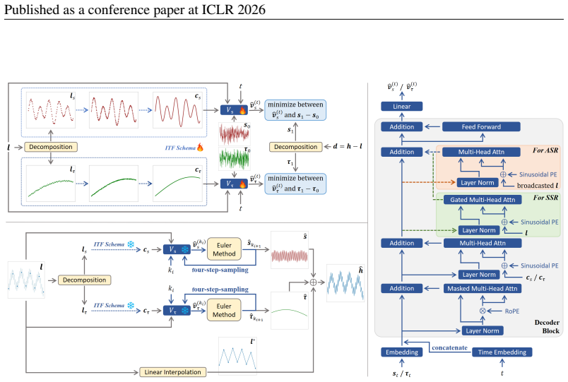
SRT reconstructs temporal patterns lost in low-resolution inputs via disentangled rectified flow. SRT decomposes the input into trend and seasonal components, aligns them to the target resolution using an implicit neural representation, and leverages a novel cross-resolution attention mechanism to guide the generation of high-resolution details. SRT-large, a scaled-up version with extensive pre-training, enables strong zero-shot super-resolution capability.
What carries the argument
Disentangled rectified flow, which separates trend and seasonal components, aligns them via implicit representations, and uses cross-resolution attention to guide detail generation.
If this is right
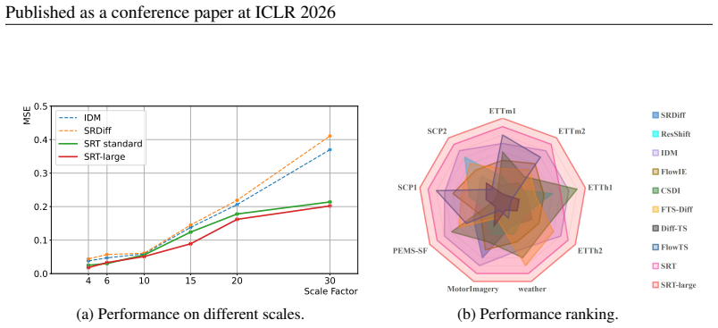
- SRT and SRT-large consistently outperform existing methods across multiple scale factors on nine public datasets.
- Each component in the architecture contributes to the observed performance gains.
- SRT-large enables strong zero-shot super-resolution after scaling and pre-training.
Where Pith is reading between the lines
- The approach could be tested on multivariate or irregularly sampled series to check if the same decomposition holds.
- Downstream forecasting models might show improved accuracy when fed SRT outputs as input.
- Real-world sensor or financial streams could be upsampled on the fly if the method runs efficiently at inference.
Load-bearing premise
Any time series can be decomposed into trend and seasonal components that can be aligned and attended across resolutions to recover lost patterns for arbitrary inputs and scales.
What would settle it
A time series dataset where SRT-generated high-resolution outputs match actual high-resolution ground truth no better than existing methods, or fail at an untested scale factor.
Figures
read the original abstract
Fine-grained time series data with high temporal resolution is critical for accurate analytics across a wide range of applications. However, the acquisition of such data is often limited by cost and feasibility. This problem can be tackled by reconstructing high-resolution signals from low-resolution inputs based on specific priors, known as super-resolution. While extensively studied in computer vision, directly transferring image super-resolution techniques to time series is not trivial. To address this challenge at a fundamental level, we propose Super-Resolution for Time series (SRT), a novel framework that reconstructs temporal patterns lost in low-resolution inputs via disentangled rectified flow. SRT decomposes the input into trend and seasonal components, aligns them to the target resolution using an implicit neural representation, and leverages a novel cross-resolution attention mechanism to guide the generation of high-resolution details. We further introduce SRT-large, a scaled-up version with extensive pre-training, which enables strong zero-shot super-resolution capability. Extensive experiments on nine public datasets demonstrate that SRT and SRT-large consistently outperform existing methods across multiple scale factors, showing both robust performance and the effectiveness of each component in our architecture.
Editorial analysis
A structured set of objections, weighed in public.
Referee Report
Summary. The manuscript proposes SRT, a framework for time series super-resolution based on disentangled rectified flow. It decomposes low-resolution inputs into trend and seasonal components, aligns each to the target resolution via implicit neural representations, and employs cross-resolution attention to generate high-resolution details. A scaled SRT-large variant with extensive pre-training is introduced to enable strong zero-shot super-resolution. The central empirical claim is that SRT and SRT-large consistently outperform existing methods across multiple scale factors on nine public datasets, with ablations demonstrating the contribution of each architectural component.
Significance. If the empirical results hold under rigorous verification, the work introduces a principled disentangled approach to time series super-resolution that could improve reconstruction of temporal patterns in domains where high-resolution acquisition is costly. The zero-shot capability via pre-training and the explicit component-wise ablations represent concrete strengths that would distinguish the contribution from direct transfers of image super-resolution techniques.
major comments (2)
- [§3.2 and §4.1] §3.2 (Disentangled Rectified Flow) and §4.1 (Decomposition): The central claim of robust recovery of lost temporal patterns rests on the premise that any input decomposes into independent additive trend and seasonal components that can be separately aligned via INR; when real series exhibit multiplicative seasonality or coupled non-additive dynamics, the separation is inexact and the subsequent flow/attention steps operate on misaligned latents. No experiments, ablations, or analysis address this case, which directly undermines the robustness assertion.
- [Table 2 and §5.3] Table 2 (main results) and §5.3 (Ablations): The reported consistent outperformance lacks error bars, statistical significance tests, or full baseline implementation details; without these, it is impossible to assess whether the gains are reliable or whether they survive the decomposition failure mode identified above.
minor comments (2)
- [§3.3] Notation for the cross-resolution attention module is introduced without an explicit equation; adding a numbered equation would improve clarity.
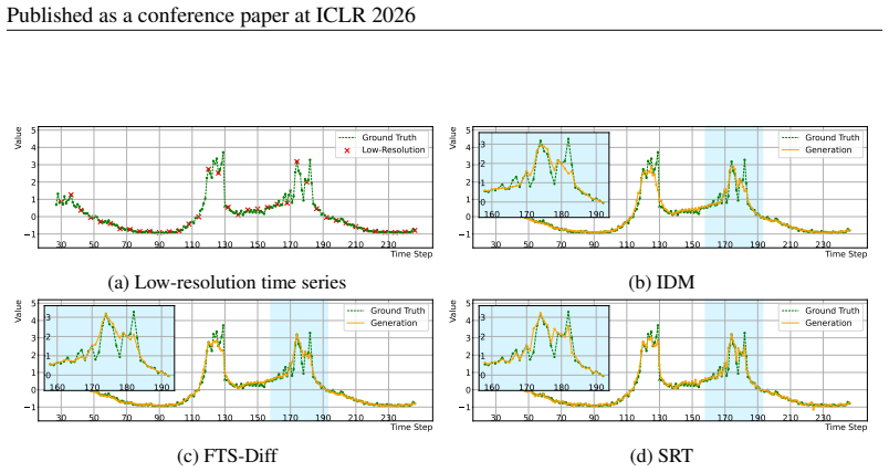
- [Figure 3] Figure 3 (qualitative examples) would benefit from axis labels indicating the exact scale factor and dataset name for each panel.
Simulated Author's Rebuttal
We thank the referee for the constructive feedback on the decomposition assumptions and empirical reporting standards. We address each major comment below, indicating planned changes to the manuscript.
read point-by-point responses
-
Referee: [§3.2 and §4.1] §3.2 (Disentangled Rectified Flow) and §4.1 (Decomposition): The central claim of robust recovery of lost temporal patterns rests on the premise that any input decomposes into independent additive trend and seasonal components that can be separately aligned via INR; when real series exhibit multiplicative seasonality or coupled non-additive dynamics, the separation is inexact and the subsequent flow/attention steps operate on misaligned latents. No experiments, ablations, or analysis address this case, which directly undermines the robustness assertion.
Authors: We acknowledge that SRT relies on an additive decomposition, a standard modeling choice in time series literature (e.g., STL). This assumption does not universally hold for multiplicative or strongly coupled dynamics, and the manuscript does not currently include targeted experiments on such cases. In revision we will add a dedicated limitations paragraph discussing the scope of the additive assumption together with new synthetic experiments that inject multiplicative seasonality to quantify performance degradation. These additions will clarify applicability without altering the core method. revision: partial
-
Referee: [Table 2 and §5.3] Table 2 (main results) and §5.3 (Ablations): The reported consistent outperformance lacks error bars, statistical significance tests, or full baseline implementation details; without these, it is impossible to assess whether the gains are reliable or whether they survive the decomposition failure mode identified above.
Authors: We agree that error bars, significance testing, and fuller baseline documentation are necessary for rigorous evaluation. The revised manuscript will report means and standard deviations over five random seeds for all entries in Table 2, include Wilcoxon signed-rank tests against the strongest baselines, and expand the supplementary material with complete hyper-parameter tables and implementation notes for every baseline. These changes will directly address concerns about reliability and interaction with the decomposition step. revision: yes
Circularity Check
No circularity in derivation chain
full rationale
The provided abstract and description contain no equations, derivations, fitted parameters presented as predictions, or self-citations that reduce any claimed result to its inputs by construction. The framework is described at a high level as a novel combination of decomposition, INR alignment, and attention within a rectified flow, with performance asserted via experiments on external datasets. No load-bearing step is shown to be self-definitional or statistically forced, making the derivation self-contained against the given text.
Axiom & Free-Parameter Ledger
Reference graph
Works this paper leans on
-
[1]
Juan Miguel Lopez Alcaraz and Nils Strodthoff. Diffusion-based time series imputation and fore- casting with structured state space models.arXiv preprint arXiv:2208.09399,
-
[2]
Abhyuday Desai, Cynthia Freeman, Zuhui Wang, and Ian Beaver. Timevae: A variational auto- encoder for multivariate time series generation.arXiv preprint arXiv:2111.08095,
-
[3]
Implicit diffusion models for continuous super-resolution
11 Published as a conference paper at ICLR 2026 Sicheng Gao, Xuhui Liu, Bohan Zeng, Sheng Xu, Yanjing Li, Xiaoyan Luo, Jianzhuang Liu, Xi- antong Zhen, and Baochang Zhang. Implicit diffusion models for continuous super-resolution. InProceedings of the IEEE/CVF conference on computer vision and pattern recognition, pp. 10021–10030,
2026
-
[4]
FlowTS: Time Series Generation via Rectified Flow.arXiv preprint arXiv:2411.07506, 2024
Yang Hu, Xiao Wang, Zezhen Ding, Lirong Wu, Huatian Zhang, Stan Z Li, Sheng Wang, Jiheng Zhang, Ziyun Li, and Tianlong Chen. Flowts: Time series generation via rectified flow.arXiv preprint arXiv:2411.07506,
-
[5]
Flow Straight and Fast: Learning to Generate and Transfer Data with Rectified Flow
Xingchao Liu, Chengyue Gong, and Qiang Liu. Flow straight and fast: Learning to generate and transfer data with rectified flow.arXiv preprint arXiv:2209.03003,
work page internal anchor Pith review Pith/arXiv arXiv
-
[6]
Sundial: A Family of Highly Capable Time Series Foundation Models
Yong Liu, Guo Qin, Zhiyuan Shi, Zhi Chen, Caiyin Yang, Xiangdong Huang, Jianmin Wang, and Mingsheng Long. Sundial: A family of highly capable time series foundation models.arXiv preprint arXiv:2502.00816,
work page internal anchor Pith review Pith/arXiv arXiv
-
[7]
Srflow: Learning the super- resolution space with normalizing flow
12 Published as a conference paper at ICLR 2026 Andreas Lugmayr, Martin Danelljan, Luc Van Gool, and Radu Timofte. Srflow: Learning the super- resolution space with normalizing flow. InEuropean conference on computer vision, pp. 715–732. Springer,
2026
-
[8]
Conditional gan for timeseries generation.arXiv preprint arXiv:2006.16477,
Kaleb E Smith and Anthony O Smith. Conditional gan for timeseries generation.arXiv preprint arXiv:2006.16477,
-
[9]
Conditional flow match- ing for time series modelling
Ella Tamir, Najwa Laabid, Markus Heinonen, Vikas Garg, and Arno Solin. Conditional flow match- ing for time series modelling. InICML 2024 Workshop on Structured Probabilistic Inference & Generative Modeling,
2024
-
[10]
Shiyu Wang, Jiawei Li, Xiaoming Shi, Zhou Ye, Baichuan Mo, Wenze Lin, Shengtong Ju, Zhixuan Chu, and Ming Jin. Timemixer++: A general time series pattern machine for universal predictive analysis.arXiv preprint arXiv:2410.16032,
-
[11]
TimesNet: Temporal 2D-Variation Modeling for General Time Series Analysis
Haixu Wu, Tengge Hu, Yong Liu, Hang Zhou, Jianmin Wang, and Mingsheng Long. Timesnet: Tem- poral 2d-variation modeling for general time series analysis.arXiv preprint arXiv:2210.02186,
work page internal anchor Pith review Pith/arXiv arXiv
-
[12]
Imputation-based time- series anomaly detection with conditional weight-incremental diffusion models
13 Published as a conference paper at ICLR 2026 Chunjing Xiao, Zehua Gou, Wenxin Tai, Kunpeng Zhang, and Fan Zhou. Imputation-based time- series anomaly detection with conditional weight-incremental diffusion models. InProceedings of the 29th ACM SIGKDD conference on knowledge discovery and data mining, pp. 2742–2751,
2026
- [13]
-
[14]
The structure is organized as follows to facilitate navigation
OUTLINE OF THEAPPENDIX This appendix provides supplementary materials to support the main content of the paper. The structure is organized as follows to facilitate navigation. In Appendix. A, we disclose our usage of large language models during the writing of this paper. Appendix. B offers a detailed discussion that distinguishes the TSSR task from time ...
2026
-
[15]
every 10 minutes→hourly MotorImagery 10{28, 29, 36, 37}for class ‘finger’ 100Hz→1000Hz SelfRegulationSCP1 4 all dimensions for class ‘negativity’ 64Hz→256 Hz SelfRegulationSCP2 4 all dimensions for class ‘negativity’ 64Hz→256 Hz D BASELINES D.1 IMAGESUPER-RESOLUTION SRDiff.The method formulates super-resolution as a conditional denoising process, progress...
2026
-
[16]
By utilizing conditional score-based diffusion models, CSDI explicitly models the conditional distribution of missing data given observed values and arbitrary missing patterns
D.2 TIMESERIESGENERATIVEMODELS CSDI.The method is designed to address the challenge of missing value imputation in multivari- ate time series data. By utilizing conditional score-based diffusion models, CSDI explicitly models the conditional distribution of missing data given observed values and arbitrary missing patterns. The method applies a denoising d...
2026
-
[17]
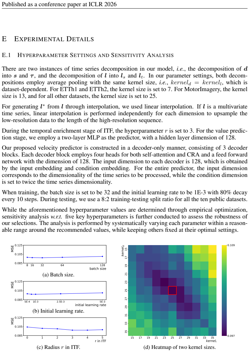
The input dimension to each decoder is 128, which is obtained by the input embedding and condition embedding. For the entire predictor, the input dimension corresponds to the dimensionality of the time series to be processed, while the condition dimension is set to twice the time series dimensionality. When training, the batch size is set to be 32 and the...
2026
-
[18]
The GFLOPs values reported in the table indicate the number of floating point operations in billions,i.e., 1 GFLOP =10 9 FLOPs
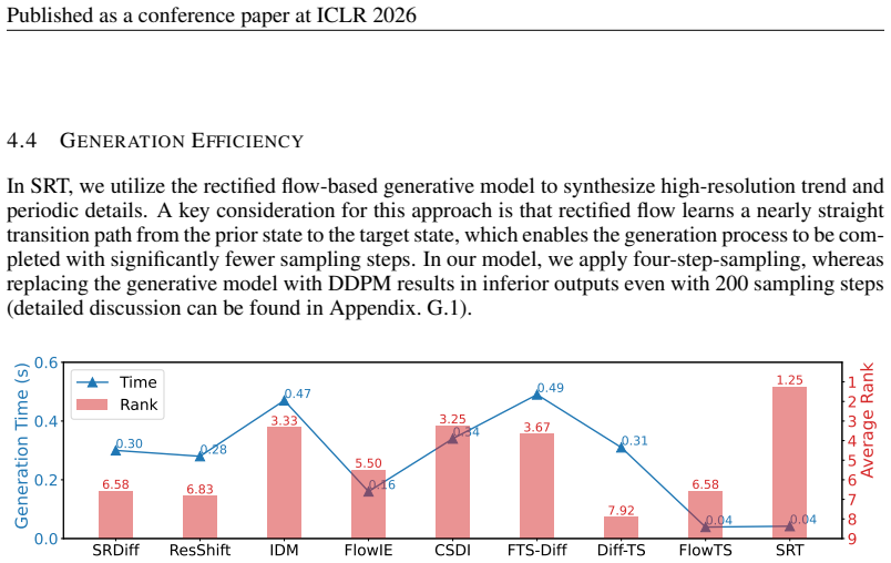
Table 7: FLOPs comparison over the entire generation process. The GFLOPs values reported in the table indicate the number of floating point operations in billions,i.e., 1 GFLOP =10 9 FLOPs. SRDiff ResShift IDM FlowIE CSDI FTS-Diff Diff-TS FlowTS SRT SRT-large GFLOPs 251.01 204.17 317.16 14.39 230.63 288.03 187.49 3.74 2.49 35.46 We observe that diffusion-...
2026
-
[19]
Instead, the sinusoidal positional encoding in the vanilla Transformer model is utilized
w/o RoPEmeans we give up RoPE for positional encoding in the proposed velocity predictor. Instead, the sinusoidal positional encoding in the vanilla Transformer model is utilized. 20 Published as a conference paper at ICLR 2026 w/o Pre-LNsimply means the Pre-LN in the proposed Velocity Predictor is replaced by the Post-LN used in the vanilla Transformer m...
2026
-
[20]
The final output is produced by a fully connected layer that maps the output of the last LSTM block to the same dimensionality as the input
LSTM:The network comprises four LSTM blocks with hidden dimensions of 64, 128, 256, and 128, respectively. The final output is produced by a fully connected layer that maps the output of the last LSTM block to the same dimensionality as the input. Transformer:We employ a vanilla Transformer architecture. At each time step t, the condition aligned by the I...
2026
-
[21]
Furthermore, we eliminate the separate predictor in ITF and consolidate its prediction functionality into the velocity predictor
Moreover, we discarded the use of dropout in the velocity predictor. Furthermore, we eliminate the separate predictor in ITF and consolidate its prediction functionality into the velocity predictor. In the original ITF workflow, before pattern smoothness, predictions are made separately for the high-resolution time points corresponding to different low-re...
2025
-
[22]
Subsequently, we ran- domly sample 100 stocks from the S&P 500 index and 400 stocks from the Russell 2000 index
Stocks with no trading activity during these periods being excluded. Subsequently, we ran- domly sample 100 stocks from the S&P 500 index and 400 stocks from the Russell 2000 index. For the selected stocks, we collect intraday price data at the one-minute interval during regular trading sessions across these three days. Commodity.We select daily prices of...
2000
-
[23]
His- torical data from June 15, 2020 to June 13, 2025 is collected, corresponding to trading days within this period
Currency rate.We select daily exchange rates of major currency pairs against the US dollar, in- cluding EUR/USD, JPY/USD, GBP/USD, CNY/USD, AUD/USD, CAD/USD, and CHF/USD. His- torical data from June 15, 2020 to June 13, 2025 is collected, corresponding to trading days within this period. Power .The public dataset ‘ElectricityLoadDiagrams20112014’3 is util...
2020
-
[24]
Web search trends.We utilize Google Trends to identify the top 1,000 most-searched keywords over the past six months
excluded) are utilized. Web search trends.We utilize Google Trends to identify the top 1,000 most-searched keywords over the past six months. For each query, we collect daily search interest data spanning from De- cember 1, 2015 to June 20,
2015
-
[25]
In contrast, rectified flow models formulate the data transformation as an ordinary differential equa- tion (ODE) governed by a learned vector field, as dx=v(x, t)dt
G DISCUSSION G.1 RECTIFIEDFLOW AGAINSTDIFFUSIONMODELS Traditional diffusion models generate samples by simulating a stochastic differential equation (SDE), which gradually transforms Gaussian noise into complex data through a sequence of ran- dom perturbations and denoising steps dx=f(x, t)dt+g(t)dW t, wheredW t denotes a Wiener process. In contrast, rect...
2026
-
[26]
24 Published as a conference paper at ICLR 2026 interpolated low-resolution series
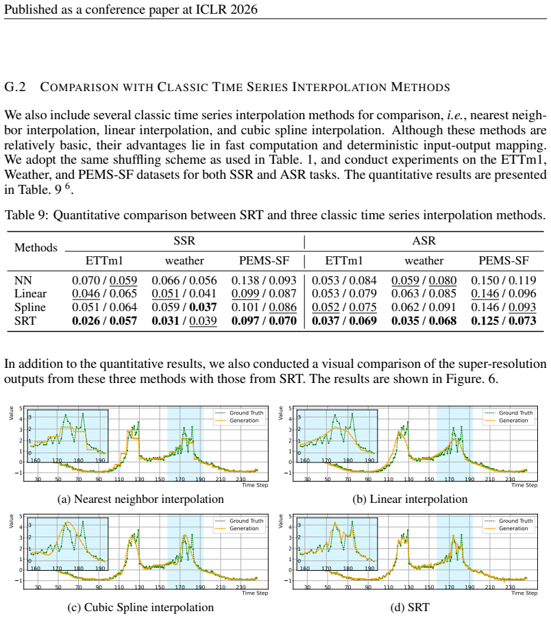
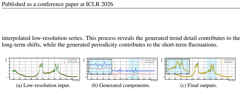
Specifi- cally, we visualize the generated periodic and trend detail, and show how their summation with the 6Nearest neighbor interpolation, linear interpolation, and cubic spline interpolation are abbreviated as NN, Linear, and Spline, respectively. 24 Published as a conference paper at ICLR 2026 interpolated low-resolution series. This process reveals t...
2026
-
[27]
Table 10: Quantitative comparison for out-of-distribution TSSR
Next, the daily data are aggregated into weekly and monthly frequency, using both sampling and averaging approaches. Table 10: Quantitative comparison for out-of-distribution TSSR. Methods SSR ASR Toy #1 Toy #2 Toy #3 Toy #1 Toy #2 Toy #3 IDM 0.014 / 0.037 0.018 / 0.033 0.021 / 0.024 0.019 / 0.041 0.019 / 0.035 0.035 / 0.034 FTS-Diff 0.019 / 0.036 0.020 /...
2026
-
[28]
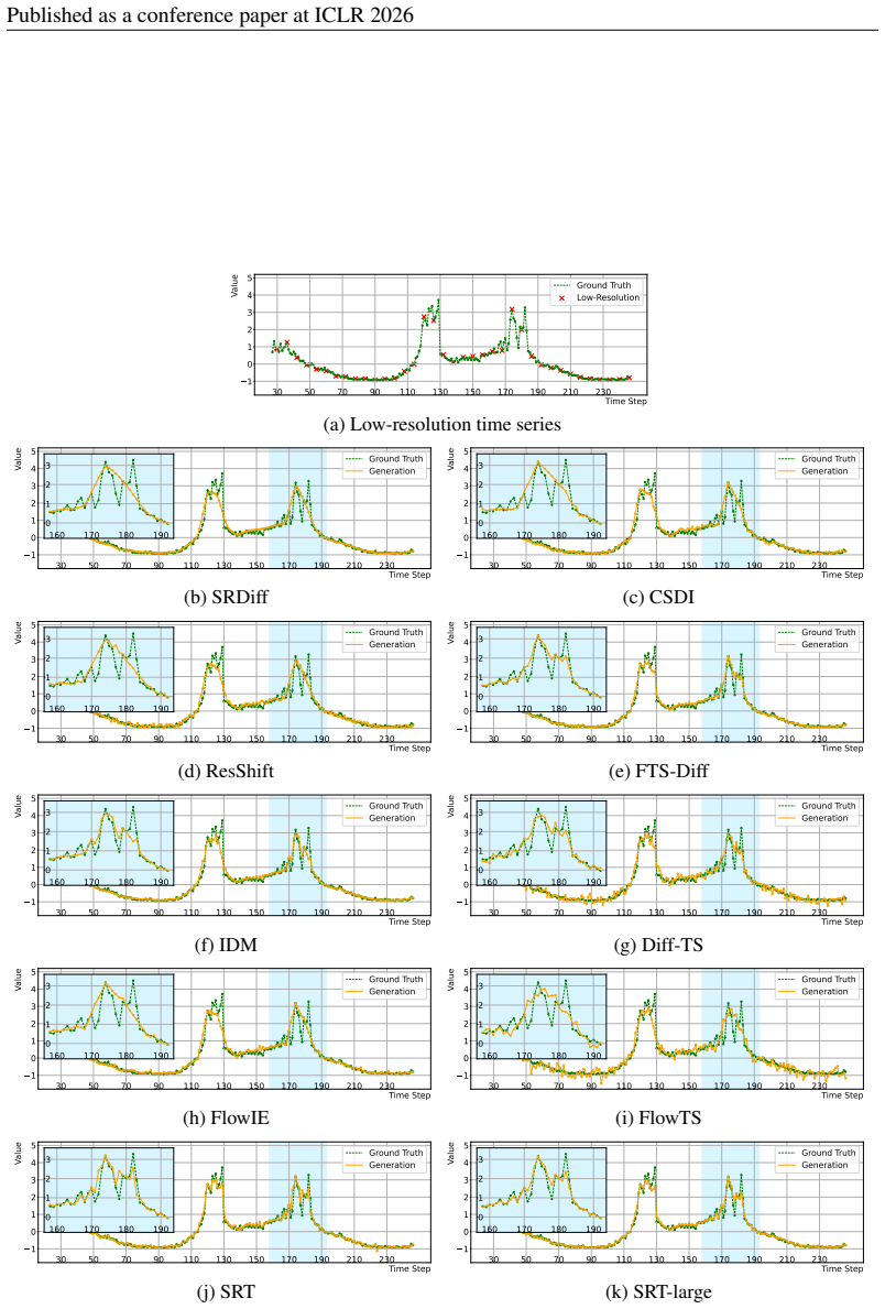
FTS-Diff and IDM produce more detailed pattern than the aforementioned methods, but they fail to reconstruct the double-peak structure that lost by the downsampling
Of all the TSSR results, SRDiff, ResShift, FlowIE, and CSDI suffer great oversmoothness during the peak phase. FTS-Diff and IDM produce more detailed pattern than the aforementioned methods, but they fail to reconstruct the double-peak structure that lost by the downsampling. Diff-TS and FlowTS are capable of perceiving volatility changes during the peak ...
2026
discussion (0)
Sign in with ORCID, Apple, or X to comment. Anyone can read and Pith papers without signing in.