Statistically Valid Hyperparameter Selection: From Tuning to Guarantees
Pith reviewed 2026-06-25 20:19 UTC · model grok-4.3
The pith
Hyperparameter selection can be performed with explicit finite-sample guarantees on reliability by framing it as multiple hypothesis testing.
A machine-rendered reading of the paper's core claim, the machinery that carries it, and where it could break.
Core claim
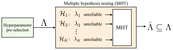
The learn-then-test (LTT) paradigm formulates hyperparameter selection as multiple hypothesis testing over a candidate set of hyperparameters. This enables the selection of hyperparameters that provably satisfy application-specific reliability requirements such as bounds on average risk, quantile risk, or information-theoretic constraints, with explicit, finite-sample control of error probabilities. The supporting statistical machinery, namely p-values, e-values, and concentration inequalities, is developed from first principles.
What carries the argument
The learn-then-test (LTT) paradigm, which formulates hyperparameter selection as multiple hypothesis testing over a candidate set to enforce reliability constraints.
If this is right
- Hyperparameters can be selected to satisfy a bound on average risk with an explicit finite-sample error probability.
- The same selection procedure applies to quantile risk and information-theoretic reliability constraints.
- The guarantees hold without asymptotic approximations and extend to any setting where valid p-values or e-values are available for the reliability metric.
- The method separates the computation of per-candidate statistics from the final multiple-testing correction.
Where Pith is reading between the lines
- The framework could be applied to other discrete selection tasks such as choosing among model architectures or data preprocessing pipelines.
- In regulated domains the explicit error control may support documentation required for safety certification.
- Efficiency gains may come from designing candidate sets or testing procedures that exploit structure in the hyperparameter space.
Load-bearing premise
Valid p-values or e-values can be computed for each hyperparameter candidate with respect to the chosen reliability metric and the multiple-testing procedure controls the relevant error rates.
What would settle it
A repeated experiment in which the selected hyperparameter violates the target reliability bound at a frequency higher than the error rate claimed by the procedure.
Figures














read the original abstract
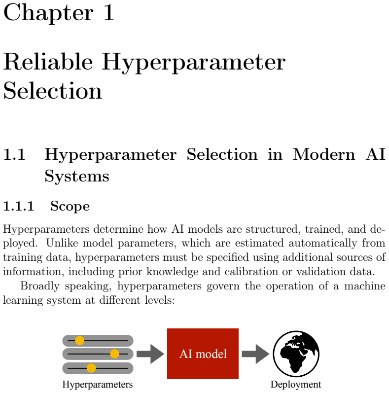
Hyperparameter selection is a critical step in the deployment of modern artificial intelligence systems, given the need to tune degrees of freedom such as inference-time parameters, implementation-level settings, and thresholds driving decision rules. Despite its practical importance, hyperparameter selection is typically performed using best-effort empirical methods such as grid search or Bayesian optimization, which provide no formal statistical guarantees on reliability or safety. This monograph presents a unified statistical framework for reliable hyperparameter selection, centered on the learn-then-test (LTT) paradigm, which formulates the problem as multiple hypothesis testing over a candidate set of hyperparameters. The framework enables the selection of hyperparameters that provably satisfy application-specific reliability requirements -- such as bounds on average risk, quantile risk, or information-theoretic constraints -- with explicit, finite-sample control of error probabilities. The supporting statistical machinery, namely p-values, e-values, and concentration inequalities, is developed from first principles in a dedicated appendix.
Editorial analysis
A structured set of objections, weighed in public.
Referee Report
Summary. The manuscript introduces the learn-then-test (LTT) paradigm, which recasts hyperparameter selection as multiple hypothesis testing over a fixed candidate set. For each candidate, valid p-values or e-values are constructed relative to a chosen reliability metric (average risk, quantile risk, or information-theoretic constraint); a multiple-testing procedure then yields a selected set of hyperparameters that provably meet the reliability requirement with explicit finite-sample error control. The required p-value/e-value constructions and concentration inequalities are stated to be supplied from first principles in a dedicated appendix.
Significance. If the p-value and e-value constructions are valid, the framework supplies the first unified, finite-sample guarantee for hyperparameter selection across multiple risk types. This directly addresses the absence of statistical validity in current tuning practice and is relevant for safety-critical deployments. The explicit development of the statistical machinery from first principles is a positive feature that supports verification and extension.
major comments (2)
- [Appendix] Appendix (p-value constructions for quantile risk): the manuscript asserts that valid p-values are supplied for the quantile-risk metric, but the specific concentration inequality or test statistic used to obtain finite-sample validity under the null is not stated in the main text or summarized; this construction is load-bearing for the claim that the framework covers quantile risk with explicit error control.
- [§3] §3 (multiple-testing step): the error-rate guarantee is stated to follow from any valid multiple-testing procedure, yet the manuscript does not specify which procedure (e.g., Bonferroni, closed testing, or e-value-based) is recommended when the reliability metric is information-theoretic; without this, the finite-sample claim for that metric remains incomplete.
minor comments (2)
- [Abstract] The abstract refers to 'a dedicated appendix' without a label (e.g., Appendix A); add the label and a one-sentence pointer from the main text to the relevant constructions.
- [§2] Notation for the reliability metrics (average risk, quantile risk, information-theoretic) should be introduced once in §2 and used consistently thereafter to avoid ambiguity when the same symbol appears in different contexts.
Simulated Author's Rebuttal
We thank the referee for the positive assessment of the LTT framework and for the constructive comments on clarity. We address each major comment below and will revise the manuscript to incorporate the suggested improvements.
read point-by-point responses
-
Referee: [Appendix] Appendix (p-value constructions for quantile risk): the manuscript asserts that valid p-values are supplied for the quantile-risk metric, but the specific concentration inequality or test statistic used to obtain finite-sample validity under the null is not stated in the main text or summarized; this construction is load-bearing for the claim that the framework covers quantile risk with explicit error control.
Authors: We agree that a high-level summary of the quantile-risk p-value construction would improve readability. The appendix derives these p-values from a concentration inequality applied to the empirical quantile estimator (a Hoeffding-style bound adapted to order statistics). In the revision we will add a one-paragraph summary of the test statistic and inequality in Section 2, while retaining the full derivation in the appendix. revision: yes
-
Referee: [§3] §3 (multiple-testing step): the error-rate guarantee is stated to follow from any valid multiple-testing procedure, yet the manuscript does not specify which procedure (e.g., Bonferroni, closed testing, or e-value-based) is recommended when the reliability metric is information-theoretic; without this, the finite-sample claim for that metric remains incomplete.
Authors: The framework is intentionally procedure-agnostic provided the chosen multiple-testing method controls the target error rate. To complete the finite-sample claim for the information-theoretic metric, the revision will explicitly recommend the Bonferroni correction (or its e-value counterpart) applied to the p-values/e-values constructed in the appendix; this choice directly yields finite-sample family-wise error control. We will also note that stronger procedures such as closed testing may be substituted when available. revision: yes
Circularity Check
No significant circularity identified
full rationale
The paper's central derivation formulates hyperparameter selection as multiple hypothesis testing over a candidate set and states that the supporting p-values, e-values, and concentration inequalities are developed from first principles in a dedicated appendix. No load-bearing step reduces a claimed prediction or guarantee to a fitted input, self-citation, or ansatz by construction. The framework is presented as self-contained against external statistical benchmarks, with the multiple-testing control and reliability metrics derived independently of the target selection result.
Axiom & Free-Parameter Ledger
Reference graph
Works this paper leans on
-
[1]
Deep Variational Information Bottleneck
Abdi, H.and L. J.Williams(2010). “Principalcomponentanalysis”. In:Wiley interdisciplinary reviews: computational statistics2.4, pp. 433–459. Alemi, A. A. et al. (2016). “Deep variational information bottleneck”. In: arXiv preprint arXiv:1612.00410. Amodei, D. et al. (2016). “Concrete problems in AI safety”. In:arXiv preprint arXiv:1606.06565. Angelopoulos...
work page internal anchor Pith review Pith/arXiv arXiv 2010
-
[2]
Mutual information neural estimation
Belghazi, M. I. et al. (2018). “Mutual information neural estimation”. In: International conference on machine learning. PMLR, pp. 531–540. Benjamini, Y. and Y. Hochberg (1995). “Controlling the false discovery rate: a practical and powerful approach to multiple testing”. In:Journal of the Royal statistical society: series B (Methodological)57.1, pp. 289–...
2018
-
[3]
Probability inequalities for the sum of independent random variables
Bennett, G. (1962). “Probability inequalities for the sum of independent random variables”. In:Journal of the American Statistical Association 57.297, pp. 33–45. Bennis, M., M. Debbah, and H. V. Poor (2018). “Ultrareliable and low- latency wireless communication: Tail, risk, and scale”. In:Proceedings of the IEEE106.10, pp. 1834–1853. Bergstra, J. and Y. ...
1962
-
[4]
On the Opportunities and Risks of Foundation Models
Bernstein, S. (1924). “On a modification of Chebyshev’s inequality and of the error formula of Laplace”. In:Ann. Sci. Inst. Sav. Ukraine, Sect. Math 1.4, pp. 38–49. Bommasani, R. (2021). “On the opportunities and risks of foundation mod- els”. In:arXiv preprint arXiv:2108.07258. Bonferroni, C. (1936). “Teoria statistica delle classi e calcolo delle proba-...
work page internal anchor Pith review Pith/arXiv arXiv doi:10.1093/acprof:oso/9780199535255.001 1924
-
[5]
Comparing three learn- then-test paradigms in a multivariate normal means problem
IEEE, pp. 1742–1751. Chakraborty, A., J. Lee, and E. Katsevich (2026). “Comparing three learn- then-test paradigms in a multivariate normal means problem”. In:arXiv preprint arXiv:2601.07764. Chernoff,H. (1952). “Ameasureofasymptoticefficiencyfortestsofahypoth- esis based on the sum of observations”. In:The Annals of Mathematical Statistics, pp. 493–507. ...
-
[6]
Deep neural networks for youtube recommendations
Covington, P., J. Adams, and E. Sargin (2016). “Deep neural networks for youtube recommendations”. In:Proceedings of the 10th ACM conference on recommender systems, pp. 191–198. Dean, J. and L. A. Barroso (2013). “The tail at scale”. In:Communications of the ACM56.2, pp. 74–80. Deb, K. (2011). “Multi-objective optimisation using evolutionary algorithms: a...
-
[7]
Mask r-cnn
Hastie, T., R. Tibshirani, J. Friedman, et al. (2009).The elements of statis- tical learning. He, K. et al. (2017). “Mask r-cnn”. In:Proceedings of the IEEE international conference on computer vision, pp. 2961–2969. Ho, J., A. Jain, and P. Abbeel (2020). “Denoising diffusion probabilistic mod- els”. In:Advances in neural information processing systems33,...
2009
-
[8]
Training Compute-Optimal Large Language Models
Ho, J. et al. (2022). “Video diffusion models”. In:Advances in neural infor- mation processing systems35, pp. 8633–8646. Hoeffding, W. (1963). “Probability inequalities for sums of bounded ran- dom variables”. In:Journal of the American statistical association58.301, pp. 13–30. Hoffmann, J. et al. (2022). “Training compute-optimal large language mod- els”...
work page internal anchor Pith review Pith/arXiv arXiv doi:10.1098/rsta.2024.0522 2022
-
[9]
Hypothesis testing with e-values
Ramdas, A. and R. Wang (2025). “Hypothesis testing with e-values”. In: Foundations and Trends®in Statistics1.1-2, pp. 1–390. Ramdas, A. et al. (2019). “A sequential algorithm for false discovery rate control on directed acyclic graphs”. In:Biometrika106.1, pp. 69–86. Ramdas, A. et al. (2023). “Game-theoretic statistics and safe anytime-valid inference”. I...
2025
-
[10]
Randomization inference: Theory and applications
Thomson/Brooks/Cole Belmont, CA. Ritzwoller, D. M., J. P. Romano, and A. M. Shaikh (2024). “Randomization inference: Theory and applications”. In:arXiv preprint arXiv:2406.09521. Sant Ana, P. M. de and N. Marchenko (2020). “Radio access scheduling using CMA-ES for optimized QoS in wireless networks”. In:2020 IEEE Globecom Workshops (GC Wkshps. IEEE, pp. 1...
-
[11]
Recursivedeepmodelsforsemanticcompositionality over a sentiment treebank
Socher,R.etal.(2013).“Recursivedeepmodelsforsemanticcompositionality over a sentiment treebank”. In:Proceedings of the 2013 conference on empirical methods in natural language processing, pp. 1631–1642. Song,Y.etal.(2026).“DemystifyingPredictionPoweredInference”.In:arXiv preprint arXiv:2601.20819. Stefani, A. G. et al. (2014). “Confidence intervals for th...
-
[12]
The information bottleneck method
MIT press Cambridge. Tibshirani, R. (1996). “Regression shrinkage and selection via the lasso”. In: Journal of the Royal Statistical Society Series B: Statistical Methodology 58.1, pp. 267–288. 143 Tishby, N., F. C. Pereira, and W. Bialek (2000). “The information bottleneck method”. In:arXiv preprint physics/0004057. Valcarce, A. (2020). “Wireless Suite: ...
work page internal anchor Pith review Pith/arXiv arXiv 1996
-
[13]
Fashion-MNIST: a Novel Image Dataset for Benchmarking Machine Learning Algorithms
Cambridge university press. Ville, J. (1939).Étude critique de la notion de collectif. Paris: Gauthier- Villars. Vovk, V. and R. Wang (2021). “E-values: Calibration, combination and ap- plications”. In:The Annals of Statistics49.3, pp. 1736–1754.doi:10 . 1214/20-AOS2020.url:https://doi.org/10.1214/20-AOS2020. Wang, R. and A. Ramdas (Jan. 2022). “False Dis...
work page internal anchor Pith review Pith/arXiv arXiv doi:10.1214/20-aos2020 1939
discussion (0)
Sign in with ORCID, Apple, or X to comment. Anyone can read and Pith papers without signing in.