REVIEW 3 major objections 8 minor 27 references
D2Q9 lattice Boltzmann cannot be second-order accurate without neglecting cubic parasitic terms; only a tuned equilibrium-plus-rate package keeps an oblique vortex dipole on track.
Reviewed by Pith at T0; open to challenge. T0 means a machine referee read the full paper against a public rubric. the ladder, T0–T4 →
T0 review · grok-4.5
2026-07-12 04:01 UTC pith:VGMDWWRO
load-bearing objection Solid D2Q9 analysis of cubic parasites plus a useful new convective isotropy test; ranking of schemes is qualitative but the core math and LB2/LB5 contrast hold up. the 3 major comments →
Isotropy and Galilean invariance of Lattice Boltzmann Method: Theoretical and numerical analysis using oblique dipole benchmark *
The pith
A machine-rendered reading of the paper's core claim, the machinery that carries it, and where it could break.
Core claim
For the D2Q9 model the second-order equivalent momentum equations contain non-vanishing cubic parasitic terms Sx and Sy. The scheme therefore cannot recover fully Galilean-invariant second-order Navier–Stokes unless those terms are neglected or reduced by a non-standard heat-flux equilibrium; the highest-moment equilibrium is invisible at second order yet controls higher-order fidelity, as demonstrated by the oblique dipole test in which truncating it destroys the coherent structures while a carefully tuned free-rate package best preserves trajectories.
What carries the argument
ABCD Taylor expansion of the MRT collision-plus-streaming operator, which produces the second-order equivalent PDEs and isolates the cubic residuals Sx, Sy; the oblique dipole benchmark then converts residual magnitude into measurable trajectory error against a spectral reference.
Load-bearing premise
Ranking schemes by visual vortex shift and three global integrals at one Reynolds number, one propagation angle, and hand-chosen free rates is enough to declare which package best preserves Galilean invariance.
What would settle it
Repeat the oblique-dipole comparison at several angles and Reynolds numbers with a quantitative anisotropy metric (for example L2 contour displacement or directional kinetic-energy spectra); if the tuned package no longer yields the smallest error, the ranking claim fails.
Editorial analysis
A structured set of objections, weighed in public.
Referee Report
Summary. The manuscript analyzes the D2Q9 lattice Boltzmann method for second-order accuracy, isotropy, and Galilean invariance. Using the ABCD Taylor-expansion method, it derives the second-order equivalent PDEs (7)–(9) and exhibits the cubic parasitic terms Sx, Sy (10)–(11) for the standard equilibrium, and the reduced forms (19)–(20) under the Dubois choice for qx, qy. It shows that the equilibrium of the highest moment h does not enter the second-order system, while the Eulerian moments control the first-order structure. Five schemes (standard MRT, modified heq, projected, Dubois equilibrium, and Dubois plus Augier-type rates) are then compared on a new periodic oblique vortex-dipole benchmark against a Fourier pseudo-spectral reference, with global integrals E, Ω, P and vorticity contours used to rank isotropy and higher-order fidelity.
Significance. The theoretical part cleanly separates Eulerian versus viscous moments and makes the cubic defects and their partial elimination explicit, consistent with prior Chapman–Enskog and ABCD analyses. The oblique dipole benchmark is a useful diagnostic: by replacing wall collisions with periodic self-advection at a controllable angle, it isolates lattice anisotropy and higher-order equilibrium effects that classical stationary tests (Taylor–Green, Poiseuille, lid-driven cavity) often mask. The demonstration that truncating nonlinear heq destroys the dipole, while Dubois equilibrium plus σq σx = 1/6 best preserves trajectories, is practically informative for MRT design. Strengths include an independent spectral reference (validated on Taylor–Green) and transparent scheme definitions in Table 1.
major comments (3)
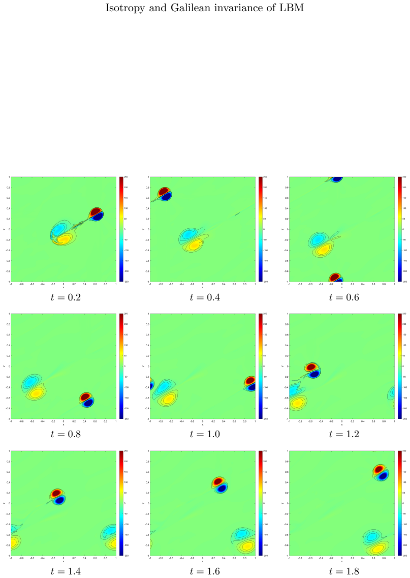
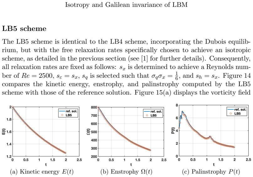
- The comparative claim that LB5 “best preserves” multi-directional isotropy and Galilean invariance (Conclusion; also §3 LB5 and abstract) rests on visual contour shift and global E/Ω/P at a single Re = 2500, single angle θ = π/6, and hand-chosen free rates (se, sq, sh). No quantitative anisotropy metric (e.g., trajectory error, angular deviation of dipole path, L2 vorticity error versus spectral reference, or multi-angle/Re sweeps) is reported. The ranking is therefore suggestive rather than conclusive; either add such metrics or temper the uniqueness language in the conclusion to match the single-configuration evidence.
- LB2 equilibrium for h is inconsistent across the manuscript: Eq. (13) and Table 1 set heq = ρ, while the LB2 numerical section states that nonlinear terms are eliminated “yielding heq = 0.” These are not equivalent. The reported collapse of the dipole and the claim that full nonlinear heq is required at higher order depend on which choice was actually implemented; the text, table, and code path must be aligned and the implemented form stated once.
- Free relaxation rates differ across schemes (LB1: se=1.9, sq=1.93, sh=1.94; LB3: se=1.99 only; LB4: se=1.9, sq=1.98, sh=1.9; LB5: σqσx=1/6 with se=sh=sx) without a controlled sensitivity study. Because the conclusion attributes LB5’s superiority jointly to Dubois equilibrium and the Augier rates, the contribution of each ingredient is not isolated; a brief ablation (Dubois with standard rates vs. standard equilibrium with Augier rates) would strengthen the causal claim.
minor comments (8)
- LB2 section: “yielding heq = 0” conflicts with Eq. (13); fix wording.
- LB3 caption/text: “compares the vorticity contours of the LB2 solution” appears to be a copy-paste error (should be LB3).
- LB4 caption: “compares the vorticity contours of the LB3 solution” should refer to LB4.
- Figure 4 layout and missing t=2.0 panel relative to the stated sequence; ensure all claimed times are shown or adjust the caption.
- Notation: Σ is called the “Hénon matrix” without a brief definition or reference for readers outside the ABCD literature; a one-line pointer would help.
- Eqs. (10)–(11) and (19)–(20): a short remark that Sx, Sy are O(Δt) and thus formally second-order defects would clarify the accuracy claim in the abstract (“cannot achieve second-order accuracy unless cubic terms are neglected”).
- References: arXiv:2411.09314 [16] is cited as preprint; update status if available at revision.
- Typos: “d’Humieres” / “d’Humières” spelling varies; “asse = 1.99” (missing space); “de computation” in the spectral section.
Circularity Check
No significant circularity: ABCD-derived parasites and external spectral benchmark are independent of the equilibria under test; mild self-citation only for method and rate choice.
specific steps
-
self citation load bearing
[§1, Table 1 and Eq. (21); LB5 description]
"Following this approach, we perform numerical investigations of these isotropic variants of the D2Q9 scheme. The corresponding relaxation parameters for LB5 scheme are selected as follows: sε = sx, sq such that σqσx = 1/6 and sh = sx."
The free rates that make LB5 'isotropic' are taken directly from the co-author Augier et al. condition without re-derivation inside the present paper; the subsequent claim that LB5 'best preserves Galilean invariance' therefore partially inherits its justification from that prior self-citation. The inheritance is mild because the ranking itself is still measured against an external spectral solution, not forced by the citation.
full rationale
The central theoretical claims (second-order equivalent PDEs (7)–(9) containing explicit cubic parasites Sx/Sy of (10)–(11) or reduced (19)–(20), and that heq drops out of second order) are obtained by applying the ABCD Taylor expansion to the D2Q9 MRT collision and the listed equilibria; the expansions are written out and do not reduce by construction to the target Galilean-invariance claim. The numerical ranking of LB1–LB5 is performed against an independent Fourier pseudo-spectral reference (integrals E, Ω, P and vorticity contours at t=1.8), not against a quantity defined by the LBM equilibria themselves. Self-citations supply the ABCD method ([7]), the projected scheme ([11]), and the Augier isotropy condition σqσx=1/6 used for LB5 rates ([1]); these are ordinary methodological inputs and do not force the dipole ranking or the existence of the parasites. No fitted parameter is renamed a prediction, no uniqueness theorem is imported to forbid alternatives, and no known empirical pattern is merely renamed. The single-angle/single-Re qualitative ranking is a limitation of strength of evidence, not circularity. Score 1 reflects only the non-load-bearing self-citation of the rate-selection rule.
Axiom & Free-Parameter Ledger
free parameters (4)
- Free MRT rates se, sq, sh (and σq via σq σx = 1/6 for LB5) =
scheme-dependent (e.g. se≈1.9–1.99; σq σx=1/6 for LB5)
- Dipole strength ωe and vortex centers / angle =
ωe=299.52838; centers given in §2; θ=π/6
- Reynolds number and viscosities via σx, σe =
Re=2500
- Grid and time-step choices (LBM 2048², Δx=Δt; spectral 1024², Δt=1e-4) =
2048² LBM; 1024² spectral
axioms (5)
- domain assumption ABCD Taylor expansion under constant acoustic scale λ=Δx/Δt yields the equivalent PDE of the MRT scheme up to the stated order (and matches Chapman–Enskog through fourth order as claimed via [7]).
- domain assumption Isothermal weakly compressible Navier–Stokes with cs=λ/√3 is the target continuum model for D2Q9 with three conserved moments.
- standard math Orthogonal d’Humières moment matrix (5) and polynomial moment hierarchy for D2Q9.
- domain assumption Pseudo-spectral integrating-factor + AB3 solution on 1024² is an accurate enough reference that residual spectral error is negligible versus LBM error at 2048².
- ad hoc to paper Periodic boundaries isolate lattice anisotropy from boundary-scheme errors.
invented entities (1)
-
Oblique Dipole Benchmark (periodic, angled self-advected vortex pair)
independent evidence
read the original abstract
This work focuses on the two-dimensional, nine-velocity (D2Q9) lattice Boltzmann model. First, we show that the D2Q9 scheme cannot achieve secondorder accuracy unless the cubic velocity terms are neglected, and we explain how some of these parasitic terms can be eliminated. Second, we demonstrate that the standard choice of the equilibrium distribution has no effect on the equivalent PDE at second order. Finally, we numerically investigate the effect of these cubic terms and study different choices of equilibrium distributions using a new benchmark called the Oblique Dipole Benchmark, which describes obliquely propagating 2D vortex dipoles with periodic boundary conditions.
Figures





Reference graph
Works this paper leans on
-
[1]
Augier, F
A. Augier, F. Dubois, B. Graille, and P. Lallemand. On rotational invariance of lattice boltzmann schemes. Computers and Mathematics with Applications , 67:239–255, 2014
2014
-
[2]
Bruneau and H
C.-H. Bruneau and H. J. H. Clercx. The normal and oblique collision of a dipole with a no-slip boundary. Computers & Fluids , 35, 2006. 18 Isotropy and Galilean invariance of LBM
2006
-
[3]
Canuto, M
C. Canuto, M. Y. Hussaini, A. Quarteroni, and T. A. Zang. Spectral Methods in Fluid Dynamics . Springer-Verlag, New York, 1988
1988
-
[4]
Canuto, M
C. Canuto, M. Y. Hussaini, A. Quarteroni, and T. A. Zang. Spectral Methods: Fundamentals in Single Domains . Springer, Berlin, 2006
2006
-
[5]
P. J. Dellar. Lattice boltzmann algorithms without cubic defects in galilean invariance on standard lattices. Journal of Computational Physics , 259:270– 283, 2014
2014
-
[6]
D’Humi` eres
D. D’Humi` eres. Generalized lattice boltzmann equations. In Rarefied Gas Dynamics: Theory and Simulations , Progress in Astronautics and Aeronautics, pages 450–458, 1992
1992
-
[7]
F. Dubois. Nonlinear fourth order taylor expansion of lattice boltzmann schemes. Asymptotic Analysis, 127:297–337, 2022
2022
-
[8]
Dubois and P
F. Dubois and P. Lallemand. Towards higher order lattice boltzmann schemes. Journal of Statistical Mechanics: Theory and Experiment , 2009:P06006, 2009
2009
-
[9]
Dubois and P
F. Dubois and P. Lallemand. On single distribution lattice boltzmann schemes for the approximation of navier stokes equations. Communications in Compu- tational Physics, 34:613–671, 2022
2022
-
[10]
Dubois, P
F. Dubois, P. Lallemand, and M. M. Tekitek. On a superconvergent lattice boltzmann boundary scheme. Comput. Math. Appl. , 59:2141–2149, 2010
2010
-
[11]
Dubois and P
F. Dubois and P. C. Philippi. Multiple relaxation times lattice boltzmann schemes with projection. Physics of Fluids , 37, 2025
2025
-
[12]
Dale R. Durran. The third-order Adams-Bashforth method: An attractive alternative to leapfrog time differencing. Monthly Weather Review, 119(3):702– 720, 1991
1991
-
[13]
Ginzbourg and P
I. Ginzbourg and P. M. Adler. Boundary flow condition analysis for the three- dimensional lattice boltzmann model. Journal of Physics II , 4:191–214, 1994
1994
-
[14]
incompressible
G. H´ azi and C. Jim´ enez. Simulation of two-dimensional decaying turbulence using the “incompressible” extensions of the lattice boltzmann method. Com- puters & Fluids , 35:280–303, 2006
2006
-
[15]
H´ azi and P
G. H´ azi and P. K´ avr´ an. On the cubic velocity deviations in lattice boltzmann methods. Journal of Physics A: Mathematical and General , 39:3127, 2006
2006
-
[16]
P. Lallemand, F. Dubois, and L.-S. Luo. Theory of the lattice boltzmann method: discrete effects due to advection. preprint, arXiv:2411.09314, 2024
Pith/arXiv arXiv 2024
-
[17]
Lallemand and L.-S
P. Lallemand and L.-S. Luo. Theory of the lattice boltzmann method: Disper- sion, dissipation, isotropy, galilean invariance, and stability. Physical Review E, 61:6546–6562, June 2000
2000
-
[18]
Latt and B
J. Latt and B. Chopard. A benchmark case for lattice boltzmann: turbulent dipole-wall collision. Int J Mod Phys C , 18:619–626, 2007
2007
-
[19]
Michelet, M
J. Michelet, M. M. Tekitek, and M. Berthier. Multiple relaxation time lattice boltzmann schemes for advection-diffusion equations with application to radar image processing. Journal of Computational Physics , 471:111612, 2022. 19 Isotropy and Galilean invariance of LBM
2022
-
[20]
Michelet, M
J. Michelet, M. M. Tekitek, and M. Berthier. Lattice boltzmann convection- diffusion model with non-constant advection velocity. Discrete and Continuous Dynamical Systems - S , 2023
2023
-
[21]
Mohammed, D
S. Mohammed, D. Graham, and T. Reis. Assessing moment-based boundary conditions for the lattice boltzmann equation: A study of dipole-wall collisions. Computers & Fluids , 176:79–96, 2018
2018
-
[22]
P. Orlandi. Vortex dipole rebound from a wall. Phys Fluids A , 2:1429–1436, 1990
1990
-
[23]
R. Peyret. Spectral Methods for Incompressible Viscous Flow. Springer-Verlag, New York, 2002
2002
-
[24]
P. C. Philippi. Personal communication, Joinville, Santa Catarina, 2018
2018
-
[25]
Y. H. Qian, D. D’Humi` eres, and P. Lallemand. Lattice BGK models for Navier- Stokes equation. Europhysics Letters, 17:479–484, 1992
1992
-
[26]
Qian and Y
Y.-H. Qian and Y. Zhou. Complete Galilean-invariant lattice BGK models for the Navier-Stokes equation. Europhysics Letters, 42:359, 1998
1998
-
[27]
R. S. Rogallo. Numerical experiments in homogeneous turbulence. Techni- cal Report NASA Technical Memorandum TM-81315, NASA Ames Research Center, 1981. 20
1981
discussion (0)
Sign in with ORCID, Apple, or X to comment. Anyone can read and Pith papers without signing in.