REVIEW 2 major objections 4 minor 66 references
A deep-learning surrogate compresses ASTEC vessel physics by over 300 imes and rolls out tens of thousands of time steps in under a minute.
Reviewed by Pith at T0; open to challenge. T0 means a machine referee read the full paper against a public rubric. the ladder, T0–T4 →
T0 review · grok-4.5
2026-07-11 19:03 UTC pith:2LPW3CGE
load-bearing objection First real multi-variable ASTEC vessel surrogate with honest metrics and open code; open-loop evaluation is the main soft spot, not a hidden fatal flaw. the 2 major comments →
A Deep Learning-based surrogate model for Severe Accidents in nuclear reactors using ASTEC
The pith
A machine-rendered reading of the paper's core claim, the machinery that carries it, and where it could break.
Core claim
An auto-encoder that maps the vessel state (1913 degrees of freedom) into a six-dimensional latent vector, coupled to a neural ODE that advances that latent state under exogenous primary-circuit boundary conditions, yields a stable, multi-variable surrogate of ASTEC's vessel physics whose wall-clock speed is hundreds of times higher than the original code.
What carries the argument
AE-NODE: a multi-branch auto-encoder that separately encodes global, plenum, core, vessel and face fields, followed by a neural ODE whose right-hand side is conditioned on the first upper-plenum and cold-leg volumes; the whole pipeline is trained with an adaptive-window teacher-forcing / autoregressive schedule.
Load-bearing premise
The vessel can be cleanly decoupled from the rest of the plant by treating the neighbouring primary-circuit volumes as fixed external inputs, without closed-loop feedback that would drive later predictions off the training manifold.
What would settle it
Couple the trained surrogate back to a live primary-circuit model (or to ASTEC itself) and check whether the closed-loop vessel predictions remain within the reported error bounds for the full duration of a severe-accident trajectory; a rapid divergence would falsify the open-loop decoupling claim.
If this is right
- Real-time operator-training simulators become feasible because a full forty-hour vessel evolution finishes in under a minute.
- The same AE-NODE architecture can be reused for other multi-physics modules once similar open-boundary data sets are generated.
- Dimensionality reduction by more than two orders of magnitude makes ensemble uncertainty quantification of severe-accident scenarios computationally practical.
- Stable multi-variable roll-outs of tens of thousands of steps demonstrate that latent neural ODEs can handle the discontinuous, stiff dynamics typical of core-melt codes.
Where Pith is reading between the lines
- If the open-loop assumption fails under closed-loop feedback, hybrid schemes that periodically re-anchor the latent state to a cheap physics residual may be required.
- The same latent-space construction could serve as a common interface for coupling independently trained surrogates of primary, secondary and containment domains.
- Because the auto-encoder already isolates the major source of error, future gains will come more from better latent reconstruction than from more sophisticated time steppers.
Editorial analysis
A structured set of objections, weighed in public.
Referee Report
Summary. The paper constructs the first (to the authors’ knowledge) purely data-driven surrogate of the ASTEC vessel domain for LOCA and SBO scenarios. An AutoEncoder compresses ~1913 degrees of freedom into a 6-dimensional latent space; a Neural ODE then advances the latent state under exogenous boundary conditions taken from the adjacent primary-circuit volumes. Separate models are trained on 700 LOCA and 286 SBO trajectories obtained by Sobol sampling of operator actions. On held-out trajectories the surrogate produces stable open-loop rollouts of 10k–50k macro-steps (4–40 h of accident time) in under a minute on CPU or GPU, simultaneously predicting ~80 scalar and field variables, with a reported wall-clock speed-up of roughly 500–900 imes relative to the ICARE module alone.
Significance. If the open-loop results hold under closed-loop coupling, the work would supply a practical building block for real-time severe-accident training simulators and would demonstrate that AE-NODE architectures can handle the multi-physics, multi-scale, discontinuous signals characteristic of integral SA codes. Strengths that should be credited include the public source code, the explicit multi-topology AE design, the adaptive-window autoregressive training schedule, the quantitative RMSE decomposition that isolates AE versus NODE error, and the frank discussion of failure modes on near-zero and highly oscillatory variables. These elements make the study a useful first benchmark even if the operational claim remains provisional.
major comments (2)
- The headline claim (Abstract; §4; Table 2) of a usable multi-hour, multi-variable surrogate is measured exclusively under open-loop forcing: at every macro-step the true ASTEC states of the first upper-plenum and cold-leg volumes are supplied as exogenous inputs (Eq. 2, §2.4, Fig. 4). Section 5.1 itself notes that even modest errors in the predicted boundary fluxes s_B1/s_B2 will alter the primary-circuit response and can drive subsequent vessel predictions off the training manifold. Because no closed-loop experiment (or even a simple one-step feedback test) is reported, the evidence does not yet support the operational claim that AE-NODE can replace the ICARE–CESAR coupling inside a real-time simulator. At minimum the authors should quantify error growth under a synthetic closed loop or clearly re-scope the claim to open-loop vessel approximation.
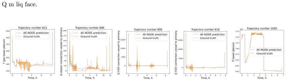
- Figures 9 and 15 show that several safety-relevant scalars (x_alpha, P_H2, m_gas, Q_liq_vap, porosity, FP mass-flow rates, and the boundary fluxes themselves) exhibit large RMSE_mean and RMSE_std while remaining low only on RMSE_max. The discussion attributes this to sharp late-time jumps and near-zero plateaus, yet no quantitative criterion is given for when a variable is considered “acceptable” for operator-training use. Without such a criterion, or without an ablation that isolates the contribution of these poorly predicted variables to the overall safety metrics, it is difficult to judge whether the surrogate is already useful or still requires substantial data filtering / capacity increases.
minor comments (4)
- Table 2 reports ASTEC times for ICARE only; the caption correctly notes this is a lower bound, but the abstract and conclusions still quote the speed-up relative to “ASTEC”. A single clarifying sentence would avoid over-statement.
- The adaptive-window schedule (Appendix E) and the precise values of the loss weights α–ω are given only in tables; a short paragraph in the main text would help reproducibility.
- Figures 26–29 illustrate the most difficult variables; adding the corresponding RMSE time series (as already done for s_B1/s_B2 in Figs. 30–31) would make the failure-mode analysis more quantitative.
- Minor notation: the same symbol S is used both for the solution manifold and for the solution space of the PDE; a brief distinction would improve readability.
Circularity Check
No circularity: purely empirical data-driven surrogate; self-citation of AE-NODE is methodological reuse, not a load-bearing derivation that forces the reported metrics.
full rationale
The paper constructs and evaluates a non-intrusive AE-NODE surrogate (AutoEncoder + Neural ODE) on ASTEC-generated LOCA/SBO trajectories. All headline claims (simultaneous prediction of ~80 vessel variables, stable 10k–50k-step autoregressive rollouts, >300 imes reduction from 1913 to 6 latent dimensions, wall-clock <1 min for ~40 h of accident time) are measured empirical outcomes on held-out test trajectories under open-loop boundary forcing (Eqs. 1–2, §2.4, Figs. 9–21, Table 2). Latent dimension λ=6, network widths, loss weights α…ω and adaptive-window schedule are free hyperparameters chosen by the authors; they do not algebraically force the reported RMSE, stability or speed-up figures. The sole self-citation ([43], same authors) supplies the base AE-NODE architecture that is then adapted (multi-domain sub-encoders, adaptive AR windows, extra loss terms). That citation is ordinary methodological reuse; the present paper’s results do not reduce to any uniqueness theorem, fitted constant or definitional identity imported from [43]. No step of the form “X derives Y but X is defined via Y”, no parameter fitted on a subset and then “predicted”, and no renaming of a known empirical pattern. The acknowledged open-loop limitation (§5.1) is a correctness/scope issue, not circularity. The derivation chain is therefore self-contained and non-circular.
Axiom & Free-Parameter Ledger
free parameters (4)
- latent dimension λ =
6
- loss weights α,β,γ,δ,ν,μ,ω =
1.0 each
- adaptive window schedule L, Nl =
L=[10,1000], Nl=[25,25]
- network widths and filter counts =
e.g. fθ layers [200,200,200,200]
axioms (4)
- domain assumption High-dimensional vessel state lives on a low-dimensional manifold that an autoencoder can learn (manifold hypothesis).
- domain assumption Operator-action vectors sampled by low-discrepancy Sobol sequences with the listed temporal constraints adequately cover the relevant accident manifold.
- ad hoc to paper Vessel dynamics can be written as a single autonomous PDE driven only by the adjacent primary-circuit volumes as exogenous inputs.
- domain assumption Neural ODEs with explicit Runge–Kutta integration can stably advance the latent state for tens of thousands of steps when trained with adaptive-window teacher-forcing + autoregressive losses.
read the original abstract
Integral codes like the Accident Source Term Evaluation Code (ASTEC) are powerful tools to study the physics of Severe Accidents (SAs) in nuclear reactors. Real time SA simulators can also be helpful in training operators of nuclear plants to react correctly to malfunctions. However, SA simulators can take up to several days per simulation, making their use infeasible for real time applications. In this work we show how to speed up a SA simulator with a fast, Deep Learning based (DL), surrogate model (SM). The SM is built as a combination of a dimensionality reduction stage, via an AutoEncoder, and a time-stepping stage, via a Neural Ordinary Differential Equation. The data on which the SM is trained are obtained from the ASTEC simulator, by sampling a set of operator actions for station blackout (SBO) and loss-of-coolant accidents (LOCA). The objective of the developed SM is to approximate multiple spatio-temporal fields for the thermal-hydraulic physics, core degradation, and fission product release modules in ASTEC's vessel domain. The SM predicts simultaneously around $80$ different physical variables (both scalar and fields), maintaining a stable autoregressive rollout up to $50$ thousand time steps. In addition, the AutoEncoder achieves a dimensionality reduction by a factor of over $300$, which allows the SM to predict up to $40$ hours of simulation in under a minute, both on CPU and GPU. This work is the first study of the capabilities and limits of DL based surrogate modeling in approximating the challenging, highly non-linear physics of ASTEC.
Figures




Reference graph
Works this paper leans on
-
[1]
Springer International Publishing, 2014
Reduced Order Methods for Modeling and Computational Reduction. Springer International Publishing, 2014. URL: http://dx.doi.org/10.1007/978-3-319-02090-7 , doi:10.1007/ 978-3-319-02090-7
-
[2]
Airbus, EDF, IMACS, ONERA, and Phimeca. Openturns. URL: https://openturns.github.io/ www/,doi:10.1007/978-3-319-11259-6_64-1
-
[3]
Sarnet, a success story
Thierry Albiol, Jean-Pierre Van Dorsselaere, and Nils Reinke. Sarnet, a success story. survey of major achievements on severe accidents and of knowledge capitalization within the astec code. 01 2008
2008
-
[4]
Universal physics transformers: A framework for efficiently scaling neural operators
Benedikt Alkin, Johannes Brandstetter, Andreas F¨ urst, Lukas Gruber, Markus Holzleitner, and Simon Schmid. Universal physics transformers: A framework for efficiently scaling neural operators. InAdvances in Neural Information Processing Systems 37, NeurIPS 2024, page 25152–25194. Neural Information Processing Systems Foundation, Inc. (NeurIPS), 2024. URL...
-
[5]
Ascher and Linda R
Uri M. Ascher and Linda R. Petzold. Computer methods for ordinary differential equations and differential-algebraic equations. 1998. URL: https://api.semanticscholar.org/CorpusID: 32366732
1998
-
[6]
The astec software system
ASNR. The astec software system. https://research-assessment.asnr.fr/ astec-software-system, 2025
2025
-
[7]
ASSAS – Artificial intelligence for simulation of severe accidents
ASSAS Consortium. ASSAS – Artificial intelligence for simulation of severe accidents. Horizon Europe Project, coordinated by ASNR, 2023-2026. 14 partners from the European Union, Switzerland and Ukraine. URL:https://assas-horizon-euratom.eu
2023
-
[8]
Layer normalization.arXiv preprint arXiv:1607.06450, 2016
Jimmy Lei Ba. Layer normalization.arXiv preprint arXiv:1607.06450, 2016
Pith/arXiv arXiv 2016
-
[9]
Joon Young Bae, Chang Hyun Song, JinHo Song, Jeong Ik Lee, Miro Seo, and Sung Joong Kim. Prediction of severe accident progression using machine learning with data-driven surrogate modeling as operator support tool.International Journal of Energy Research, 2026(1), January 2026. URL: http://dx.doi.org/10.1155/er/1416259,doi:10.1155/er/1416259
-
[10]
Representation equivalent neural operators: a framework for alias-free operator learning
Francesca Bartolucci, Emmanuel de Bezenac, Bogdan Raonic, Roberto Molinaro, Siddhartha Mishra, and Rima Alaifari. Representation equivalent neural operators: a framework for alias-free operator learning. InThirty-seventh Conference on Neural Information Processing Systems, 2023. URL: https://openreview.net/forum?id=7LSEkvEGCM
2023
-
[11]
Cristian Bodnar, Wessel P. Bruinsma, Ana Lucic, Megan Stanley, Anna Allen, Johannes Brandstetter, Patrick Garvan, Maik Riechert, Jonathan A. Weyn, Haiyu Dong, Jayesh K. Gupta, Kit Thambiratnam, Alexander T. Archibald, Chun-Chieh Wu, Elizabeth Heider, Max Welling, Richard E. Turner, and Paris Perdikaris. A foundation model for the earth system.Nature, 641(...
-
[12]
Worrall, and Max Welling
Johannes Brandstetter, Daniel E. Worrall, and Max Welling. Message passing neural PDE solvers. InInternational Conference on Learning Representations, 2022. URL: https://openreview.net/ forum?id=vSix3HPYKSU
2022
-
[13]
Report on the modelling strategy
Jure Brence, Saso Dzeroski, and Bastien Poubeau. Report on the modelling strategy. Technical report, ASSAS, May 2024. URL: https://assas-horizon-euratom.eu/wp-content/uploads/2024/11/ Report-on-modelling-strategySigned.pdf
2024
-
[14]
Steven L. Brunton and J. Nathan Kutz. Promising directions of machine learning for partial differential equations.Nature Computational Science, 4(7):483–494, June 2024. URL: http://dx. doi.org/10.1038/s43588-024-00643-2,doi:10.1038/s43588-024-00643-2
-
[15]
Steven L. Brunton, Joshua L. Proctor, and J. Nathan Kutz. Discovering governing equations from data by sparse identification of nonlinear dynamical systems.Proceedings of the National Academy of Sciences, 113(15):3932–3937, March 2016. URL: http://dx.doi.org/10.1073/pnas.1517384113, doi:10.1073/pnas.1517384113. 25
-
[16]
Mattia Cenedese, Joar Ax˚ as, Bastian B¨ auerlein, Kerstin Avila, and George Haller. Data-driven modeling and prediction of non-linearizable dynamics via spectral submanifolds.Nature Com- munications, 13(1), February 2022. URL: http://dx.doi.org/10.1038/s41467-022-28518-y , doi:10.1038/s41467-022-28518-y
-
[17]
Overview of ASTEC integral code status and perspectives
Lionel Chailan, Loic Bosland, Laure Car´ enini, Julien Chambarel, Frederic Cousin, et al. Overview of ASTEC integral code status and perspectives. In9th European Review Meeting on Severe Accident Research (ERMSAR2019), Prague, Czech Republic, March 2019.doi:irsn-04106726
2019
-
[18]
Chatelard, Joelle Fleurot, Olivier Marchand, and Patrick Drai
P. Chatelard, Joelle Fleurot, Olivier Marchand, and Patrick Drai. Assessment of icare/cathare v1 severe accident code. 07 2006.doi:10.1115/ICONE14-89307
-
[19]
P. Chatelard, N. Reinke, S. Arndt, S. Belon, L. Cantrel, L. Carenini, K. Chevalier-Jabet, F. Cousin, J. Eckel, F. Jacq, C. Marchetto, C. Mun, and L. Piar. Astec v2 severe accident integral code main features, current v2.0 modelling status, perspectives.Nuclear Engineering and De- sign, 272:119–135, June 2014. URL: http://dx.doi.org/10.1016/j.nucengdes.201...
-
[20]
Bertrand Cheynet, Patricia Chaud, Pierre-Yves Chevalier, Evelyne Fischer, Paul Mason, and Mike Mignanelli. NUCLEA - Thermodynamic properties and phase equilibria in nuclear systems.Journal de Physique IV Proceedings, 113:61 – 64, January 2004. URL: https://hal.univ-grenoble-alpes. fr/hal-01895657,doi:10.1051/jp4:20040014
-
[21]
Autoencoder diagrams
Keenan Crane. Autoencoder diagrams. https://cs.cmu.edu/~kmcrane/AutoencoderDiagrams. zip
-
[22]
P. Drai, N. Girault, L. Car´ enini, L. Laborde, J.A. Zambaux, L. Cloarec, E. Delaume, F. Fichot, C. Marchetto, S. M. O. Souvi, O. Coindreau, F. Virot, M. Jobelin, G. Astier, F. Kremer, K. Chevalier- Jabet, L. Bosland, H. Bloch, L. Chailan, R. Monod, M. Johnson, L. Foucher, A. Bleyer, A. Commande, J.J. Ingremeau, and M. Szogradi. ASTEC V3: A Comprehensive ...
2025
-
[23]
Koeberg switchboard, switchboard components and plant ca- bling evaluation for long-term operation
Eskom Holdings SOC Ltd. Koeberg switchboard, switchboard components and plant ca- bling evaluation for long-term operation. Technical Report 32-T-IPDK-008, Eskom, 2021. URL: https://www.eskom.co.za/wp-content/uploads/2024/04/32-T-IPDK-008_Koeberg_ Switchboard_Switchboard_Components_and_Plant_Cabling_Evaluation_for_LTO.pdf
2021
-
[24]
Testing the manifold hypothesis
Charles Fefferman, Sanjoy Mitter, and Hariharan Narayanan. Testing the manifold hypothesis. Journal of the American Mathematical Society, 29(4):983–1049, February 2016. URL: http://dx. doi.org/10.1090/jams/852,doi:10.1090/jams/852
doi:10.1090/jams/852 2016
-
[25]
Nicola Rares Franco, Stefania Fresca, Filippo Tombari, and Andrea Manzoni. Deep learning-based surrogate models for parametrized pdes: Handling geometric variability through graph neural networks.Chaos: An Interdisciplinary Journal of Nonlinear Science, 33(12), December 2023. URL: http://dx.doi.org/10.1063/5.0170101,doi:10.1063/5.0170101
-
[26]
A comprehensive deep learning-based approach to reduced order modeling of nonlinear time-dependent parametrized pdes.Journal of Scientific Computing, 87:1–36, 2021
Stefania Fresca, Luca Dede’, and Andrea Manzoni. A comprehensive deep learning-based approach to reduced order modeling of nonlinear time-dependent parametrized pdes.Journal of Scientific Computing, 87:1–36, 2021
2021
-
[27]
Rudy Geelen, Laura Balzano, Stephen Wright, and Karen Willcox. Learning physics-based reduced-order models from data using nonlinear manifolds.Chaos: An Interdisciplinary Jour- nal of Nonlinear Science, 34(3), March 2024. URL: http://dx.doi.org/10.1063/5.0170105, doi:10.1063/5.0170105
-
[28]
MIT Press, 2016
Ian Goodfellow, Yoshua Bengio, and Aaron Courville.Deep Learning. MIT Press, 2016. http: //www.deeplearningbook.org
2016
-
[29]
Vectorized Conditional Neural Fields: A framework for solving time-dependent parametric partial differential equations
Jan Hagnberger, Marimuthu Kalimuthu, Daniel Musekamp, and Mathias Niepert. Vectorized Conditional Neural Fields: A framework for solving time-dependent parametric partial differential equations. In Ruslan Salakhutdinov, Zico Kolter, Katherine Heller, Adrian Weller, Nuria Oliver, 26 Jonathan Scarlett, and Felix Berkenkamp, editors,Proceedings of the 41st I...
2024
-
[30]
Towards a definition of disentangled representations.arXiv preprint arXiv:1812.02230, 2018
Irina Higgins, David Amos, David Pfau, Sebastien Racaniere, Loic Matthey, Danilo Rezende, and Alexander Lerchner. Towards a definition of disentangled representations.arXiv preprint arXiv:1812.02230, 2018
Pith/arXiv arXiv 2018
-
[31]
Current State of Knowledge
Didier Jacquemain, Gerard Cenerino, Francois Corenwinder, Emmanuel IRSN Raimond, Ahmed Bentaib, Herve Bonneville, Bernard Clement, Michel Cranga, Florian Fichot, Vincent Koundy, and et al.Nuclear power reactor core melt accidents. Current State of Knowledge. EDP Sciences, Nov 2015
2015
-
[32]
Petr Karnakov, Sergey Litvinov, and Petros Koumoutsakos. Solving inverse problems in physics by optimizing a discrete loss: Fast and accurate learning without neural networks.PNAS Nexus, 3(1), December 2023. URL: http://dx.doi.org/10.1093/pnasnexus/pgae005, doi:10.1093/ pnasnexus/pgae005
-
[33]
Nitish Shirish Keskar, Dheevatsa Mudigere, Jorge Nocedal, Mikhail Smelyanskiy, and Ping Tak Peter Tang. On large-batch training for deep learning: Generalization gap and sharp minima.ArXiv, abs/1609.04836, 2016. URL:https://api.semanticscholar.org/CorpusID:5834589
Pith/arXiv arXiv 2016
-
[34]
Adam: A method for stochastic optimization.arXiv preprint arXiv:1412.6980, 2014
Diederik P Kingma and Jimmy Ba. Adam: A method for stochastic optimization.arXiv preprint arXiv:1412.6980, 2014
Pith/arXiv arXiv 2014
-
[35]
Space-time continuous PDE forecasting using equivariant neural fields
David M Knigge, David Wessels, Riccardo Valperga, Samuele Papa, Jan-Jakob Sonke, Erik J Bekkers, and Stratis Gavves. Space-time continuous PDE forecasting using equivariant neural fields. InThe Thirty-eighth Annual Conference on Neural Information Processing Systems, 2024. URL: https://openreview.net/forum?id=wN5AgP0DJ0
2024
-
[36]
Neural operator: Learning maps between function spaces with applications to pdes.Journal of Machine Learning Research, 24(89):1–97, 2023
Nikola Kovachki, Zongyi Li, Burigede Liu, Kamyar Azizzadenesheli, Kaushik Bhattacharya, Andrew Stuart, and Anima Anandkumar. Neural operator: Learning maps between function spaces with applications to pdes.Journal of Machine Learning Research, 24(89):1–97, 2023. URL: http: //jmlr.org/papers/v24/21-1524.html
2023
-
[37]
Jonas Kusch and Pia Stammer. A robust collision source method for rank adaptive dynamical low-rank approximation in radiation therapy.ESAIM: Mathematical Modelling and Numerical Analysis, 57(2):865–891, March 2023. URL: http://dx.doi.org/10.1051/m2an/2022090, doi: 10.1051/m2an/2022090
-
[38]
Kookjin Lee and Kevin T. Carlberg. Model reduction of dynamical systems on nonlinear manifolds using deep convolutional autoencoders.Journal of Computational Physics, 404:108973, March 2020. URL:http://dx.doi.org/10.1016/j.jcp.2019.108973,doi:10.1016/j.jcp.2019.108973
-
[39]
Yeonha Lee, Seok Ho Song, Joon Young Bae, Kyusang Song, Mi Ro Seo, Sung Joong Kim, and Jeong Ik Lee. Surrogate model for predicting severe accident progression in nuclear power plant using deep learning methods and rolling-window forecast.Annals of Nuclear Energy, 208:110816, December 2024. URL: http://dx.doi.org/10.1016/j.anucene.2024.110816, doi:10.1016...
-
[40]
Longze Li, Yapei Zhang, Wenxi Tian, Guanghui Su, and Suizheng Qiu. Maap5 simulation of the pwr severe accident induced by pressurizer safety valve stuck-open accident.Progress in Nuclear Energy, 77:141–151, November 2014. URL: http://dx.doi.org/10.1016/j.pnucene.2014.06.014, doi:10.1016/j.pnucene.2014.06.014
-
[41]
Fourier neural operator with learned deformations for pdes on general geometries.Journal of Machine Learning Research, 24(388):1–26, 2023
Zongyi Li, Daniel Zhengyu Huang, Burigede Liu, and Anima Anandkumar. Fourier neural operator with learned deformations for pdes on general geometries.Journal of Machine Learning Research, 24(388):1–26, 2023. URL:http://jmlr.org/papers/v24/23-0064.html
2023
-
[42]
Fourier neural operator for parametric partial differential equations
Zongyi Li, Nikola Borislavov Kovachki, Kamyar Azizzadenesheli, Burigede liu, Kaushik Bhat- tacharya, Andrew Stuart, and Anima Anandkumar. Fourier neural operator for parametric partial differential equations. InInternational Conference on Learning Representations, 2021. URL: https://openreview.net/forum?id=c8P9NQVtmnO. 27
2021
-
[43]
Alessandro Longhi, Danny Lathouwers, and Zolt´ an Perk´ o. Latent space modeling of parametric and time-dependent pdes using neural odes.Computer Methods in Applied Mechanics and Engineering, 448:118394, January 2026. URL: http://dx.doi.org/10.1016/j.cma.2025.118394, doi:10.1016/ j.cma.2025.118394
-
[44]
J. L. Lumley. The structure of inhomogeneous turbulence. In A. M. Yaglom and V. I. Tatarski, editors,Atmospheric Turbulence and Wave Propagation. Nauka, Moscow, 1967
1967
-
[45]
Andrea Malizia, Andrea Chierici, Sergio Biancotto, Marco D’Arienzo, Gian Marco Ludovici, Francesco d’Errico, Guglielmo Manenti, and Fabio Marturano. The hotspot code as a tool to improve risk analysis during emergencies: Predicting i-131 and cs-137 dispersion in the fukushima nuclear accident.International Journal of Safety and Security Engineering, 11(4)...
-
[46]
Guglielmo Padula, Michele Girfoglio, and Gianlugi Rozza. A brief review of reduced order models using intrusive and non-intrusive techniques.PAMM, 24(4), November 2024. URL: http://dx.doi. org/10.1002/pamm.202400210,doi:10.1002/pamm.202400210
-
[47]
Users’ expectations – simulator specifications
Isabel Parrado-Rodriguez. Users’ expectations – simulator specifications. WP6 Report Version 1, ASSAS, February 2024
2024
-
[48]
Film: Visual reasoning with a general conditioning layer
Ethan Perez, Florian Strub, Harm De Vries, Vincent Dumoulin, and Aaron Courville. Film: Visual reasoning with a general conditioning layer. InProceedings of the AAAI conference on artificial intelligence, volume 32, 2018
2018
-
[49]
Radaideh, Connor Pigg, Tomasz Kozlowski, Yujia Deng, and Annie Qu
Majdi I. Radaideh, Connor Pigg, Tomasz Kozlowski, Yujia Deng, and Annie Qu. Neural-based time series forecasting of loss of coolant accidents in nuclear power plants.Expert Systems with Applications, 160:113699, December 2020. URL: http://dx.doi.org/10.1016/j.eswa.2020.113699, doi:10. 1016/j.eswa.2020.113699
-
[50]
M. Raissi, P. Perdikaris, and G.E. Karniadakis. Physics-informed neural networks: A deep learning framework for solving forward and inverse problems involving nonlinear partial differential equations. Journal of Computational Physics, 378:686–707, February 2019. URL: http://dx.doi.org/10. 1016/j.jcp.2018.10.045,doi:10.1016/j.jcp.2018.10.045
-
[51]
Convolutional neural operators for robust and accurate learning of pdes.Advances in Neural Information Processing Systems, 36:77187–77200, 2023
Bogdan Raonic, Roberto Molinaro, Tim De Ryck, Tobias Rohner, Francesca Bartolucci, Rima Alaifari, Siddhartha Mishra, and Emmanuel de B´ ezenac. Convolutional neural operators for robust and accurate learning of pdes.Advances in Neural Information Processing Systems, 36:77187–77200, 2023
2023
-
[52]
D. Tarabelli, G. Ratel, R. P´ elisson, G. Guillard, M. Barnak, and P. Matejovic. Astec application to in-vessel corium retention.Nuclear Engineering and Design, 239(7):1345–1353, 2009. URL: http: //dx.doi.org/10.1016/j.nucengdes.2009.02.021,doi:10.1016/j.nucengdes.2009.02.021
-
[53]
Organized by ASNR (Autorit´ e de Sˆ uret´ e Nucl´ eaire et de Radioprotection)
Training Course, Aix-en-Provence, France.ASTEC (Accident Source Term Evaluation Code) Software: Models, Numerical Structure, Data Management, January 23–28 2023. Organized by ASNR (Autorit´ e de Sˆ uret´ e Nucl´ eaire et de Radioprotection)
2023
-
[54]
U.S. NRC. TRACE v5.840 Theory Manual: Field Equations, Solution Methods, and Physical Models. Theory manual, US Nuclear Regulatory Commission, Washington, D.C., United States, 2013
2013
-
[55]
Pauli Virtanen, Ralf Gommers, Travis E. Oliphant, Matt Haberland, Tyler Reddy, David Cournapeau, Evgeni Burovski, Pearu Peterson, Warren Weckesser, Jonathan Bright, St´ efan J. van der Walt, Matthew Brett, Joshua Wilson, K. Jarrod Millman, Nikolay Mayorov, Andrew R. J. Nelson, Eric Jones, Robert Kern, Eric Larson, C J Carey, ˙Ilhan Polat, Yu Feng, Eric W....
-
[56]
S. Wiewel, M. Becher, and N. Thuerey. Latent space physics: Towards learning the temporal evolution of fluid flow.Computer Graphics Forum, 38(2):71–82, May 2019. URL: http://dx.doi. org/10.1111/cgf.13620,doi:10.1111/cgf.13620. 28
-
[57]
Yuxin Wu and Kaiming He. Group normalization. InComputer Vision – ECCV 2018: 15th European Conference, Munich, Germany, September 8-14, 2018, Proceedings, Part XIII, page 3–19, Berlin, Heidelberg, 2018. Springer-Verlag.doi:10.1007/978-3-030-01261-8_1. 29 Table 3: Variables belonging tos g,s p,s B1 ands B2 State space Variables sg H2 cumulated mass in the ...
-
[58]
The idea behind this is that the latent spaceEneeds to be shaped before the dynamics can be approximated
we choose a low value for l = l0, typically l0 = 25, and we only train the AutoEncoder for a number NAE of epochs on Ml0 tr, i.e., we set δ = ν = µ = ω = 0.0 from Ltot. The idea behind this is that the latent spaceEneeds to be shaped before the dynamics can be approximated
-
[59]
This is done for NT F epochs
we keep Ml0 tr and we switch on the LT F and Ltm losses, while keeping ν = ω = 0, i.e., we do not train yet autoregressively. This is done for NT F epochs. The reason why we do so is to start building upf θ in the easiest possible setting; 33 Table 8: Hyper-parameters of AR training NAE NT F L N l LOCA 25 10 [10,1000] [25,25] SBO 25 10 [10,1000] [25,25]
-
[60]
We wait Nl0 epochs and after that we reshape the dataset into Ml1 tr, where l1 > l 0 and we train on Ml1 tr for Nl1 epochs
we start with Ml0 tr and we switch on also the AR losses LAR and Lf ull AR . We wait Nl0 epochs and after that we reshape the dataset into Ml1 tr, where l1 > l 0 and we train on Ml1 tr for Nl1 epochs. We repeat this process up to a certain li with the waiting times and each li pre-defined before the training starts. Thus, prior to the training, we have to...
-
[61]
The latent vector is concatenated with the flattened vector p(ˆx, tj i |kj), resulting in a concatenated vector of dimensionλ+d h1 +d c1
simple concatenation. The latent vector is concatenated with the flattened vector p(ˆx, tj i |kj), resulting in a concatenated vector of dimensionλ+d h1 +d c1
-
[62]
FiLM [48] application. The latent vector is transformed as ε→β f ilm θ (p) ⊙ε + δf ilm θ (p), where βf ilm θ : Sp →R λ and δf ilm θ : Sp →R λ are two linear transformations parametrized by weights found during training.⊙is the point-wise (Hadamard product). We did not find noticeable difference in the application of the two, so for simplicity we use conca...
-
[63]
RMSE j m = 1 Fj −1 PFj −1 i=1 ||˜s(xm,ti+1|kj)−sm(xm,ti+1|kj)||2 2 |Ωm| 1 2 ∈R dm
-
[64]
RMSE j m,mean = RMSEj m Mean{sm(xm,ti|kj)} Fj i=1 ∈R dm
-
[65]
RMSE j m,max = RMSEj m Max{sm(xm,ti|kj)} Fj i=1 ∈R dm
-
[66]
So each metric is a vector containing dm errors, each associated to a variable belonging to sm
RMSE j m,std = RMSEj m Std{sm(xm,ti|kj)} Fj i=1 ∈R dm where the index m∈ {g, p, cr, v, B 1, B2} as defined in Subsection 2.2 and ˜s(xm, ti+1|kj) can be either ˜sm i+1,1(xm, ti+1|kj), i.e., the actual prediction of AE-NODE, or ψ◦φ (sm(xm, ti+1|kj)), i.e., a simple autoencoding, as done in Figures 15 and 9. So each metric is a vector containing dm errors, e...
discussion (0)
Sign in with ORCID, Apple, or X to comment. Anyone can read and Pith papers without signing in.