REVIEW 2 major objections 5 minor 18 references
Posterior collapse has two coupled causes; one asymmetric sampling fix equalizes latent variances and restores the code.
Reviewed by Pith at T0; open to challenge. T0 means a machine referee read the full paper against a public rubric. the ladder, T0–T4 →
T0 review · grok-4.5
2026-07-11 06:14 UTC pith:5VXYHO73
load-bearing objection Clean two-cause framing and a one-line asymmetric reparameterization that actually equalizes variances; the non-ELBO status of L_λ is real but the paper already treats generation as a δ-controlled tradeoff rather than a free lunch. the 2 major comments →
λ-VAE: Variance Equalization for Posterior Collapse
The pith
A machine-rendered reading of the paper's core claim, the machinery that carries it, and where it could break.
Core claim
Posterior collapse arises from two logically independent but coupled causes—gradient imbalance, in which the reconstruction gradient decays faster than the KL force as σ_i→1, and information gap, in which sampling discards encoder signal and is algebraically identical to aggregate–prior mismatch. A single modification, sampling z=μ+σ^λϵ while retaining the KL penalty on the original σ², shifts the stable attractor to σ^*=λ^{−1/(λ−1)}, equalizes variances across dimensions, and recovers latent information capacity and reconstruction quality.
What carries the argument
Variance equalization via asymmetric reparameterization: noise is scaled by a per-dimension exponent λ while KL still uses the original posterior variance. The resulting force drives every dimension to the same equilibrium σ^*=λ^{−1/(λ−1)}; a closed-form optimal λ* follows from a net information-gain objective with one tradeoff hyperparameter δ.
Load-bearing premise
The method samples from a distribution whose variance is σ to the power 2λ while charging the KL term as if the variance were still σ squared, so the objective is no longer a standard variational lower bound on the data likelihood.
What would settle it
Train matched architectures with fixed λ=1 versus the optimal per-dimension λ* schedule on CIFAR-10 (or PixelCNN); if active-unit counts, SNR capacity, decoder capacity, and BPD fail to separate as reported (no roughly 2.8× capacity gain and no multi-fold decoder-capacity gap at near-identical BPD), the claimed mechanism is falsified.
If this is right
- Collapsed latent dimensions can be driven near zero without changing the ELBO objective or adding parameters.
- Information capacity can rise by up to 2.8× and reconstruction by up to +0.33 BPD once posterior variances are equalized.
- BPD alone is an unreliable collapse diagnostic: models can share nearly identical BPD while differing several-fold in decoder capacity allocated to the latent code.
- A single hyperparameter δ explicitly trades reconstruction fidelity against generation quality under the same prior.
- The same per-channel noise calibration principle is expected to apply to hierarchical VAEs and other stochastic bottlenecks whose noise is set globally.
Where Pith is reading between the lines
- Because the sampling and KL variances differ, generation quality can degrade when δ is set too aggressively and the aggregate posterior drifts from the prior; δ calibration is therefore load-bearing for any generative use.
- The information-gap / marginal-mismatch duality supplies a cheap, per-batch proxy for aggregate posterior quality that could replace expensive MMD or adversarial matching in other models.
- Per-dimension attractors may be more efficient than global KL reweighting (β-VAE, free bits) precisely because they act only where signal is weak.
- The same idea—set bottleneck noise to local signal strength rather than a uniform budget—likely extends to discrete latents and diffusion-style posteriors.
Editorial analysis
A structured set of objections, weighed in public.
Referee Report
Summary. The paper argues that posterior collapse in VAEs has two coupled causes—gradient imbalance (Prop. 1: reconstruction gradient decays as O((1−σ_i)^α) with α>1 so the ratio ρ_i→0 as σ_i→1) and an information gap from the stochastic bottleneck (Prop. 2), algebraically linked to aggregate–prior mismatch via Eq. 8. It proposes λ-VAE: sample z=μ+σ^λ ϵ while retaining the KL on the original σ² (Eqs. 9–10). This asymmetry is claimed to rebalance gradients, close the information gap, and drive every dimension to a common stable attractor σ^*=λ^{−1/(λ−1)} (“variance equalization”). A closed-form per-dimension λ* follows from maximizing a net-information-gain objective J with a single tradeoff hyperparameter δ. Experiments on synthetic mixtures, Binary MNIST/Omniglot, CIFAR-10 and CelebA-64 report fewer collapsed units, up to 2.8× SNR capacity, and up to +0.33 BPD, with a PixelCNN ablation showing near-identical BPD but 6.2× higher decoder capacity allocated to z.
Significance. If the analysis and method hold, the paper supplies a useful mechanistic account of collapse (gradient ratio + information-gap duality) and a lightweight, per-dimension intervention that does not alter the training objective or add parameters. The closed-form λ* (Prop. 3 / App. B.2), the stability argument for σ*, the synthetic isolation of the two causes, and the multi-architecture empirical suite (MLP, asymmetric ResNet, PixelCNN) are concrete strengths. The PixelCNN result is especially informative: it shows that BPD can mask near-total latent bypass. The work is therefore of practical interest for VAE training and of conceptual interest for any stochastic bottleneck whose noise is set globally rather than per-channel.
major comments (2)
- Eqs. 9–10 define L_λ with sampling distribution N(μ, diag(σ^{2λ})) while the KL term is evaluated under N(μ, diag(σ²)). Consequently L_λ is not a standard ELBO / variational lower bound on log p(x). The manuscript never states what quantity is being optimized, nor proves that the fixed-point encoder still yields a valid approximate posterior for ancestral sampling from the prior. All capacity/BPD gains and the variance-equalization attractor are therefore properties of a non-standard surrogate; the generation side of the δ tradeoff can fail even while reconstruction metrics improve. This is load-bearing for the claim that λ-VAE “resolves” collapse while remaining a VAE and must be addressed (e.g., by characterizing the bound, reporting prior-sample metrics systematically, or reframing the method as a regularized autoencoder).
- Section 6.3 / Figure 5 already shows that aggressive δ (e.g., 1.01) improves reconstruction while substantially degrading prior-sample ELBO (−2167 vs −1776). The abstract and conclusion nevertheless present reconstruction and capacity gains as the primary success metrics. A clearer statement of the reconstruction–generation Pareto front, and of the regime in which the asymmetric q remains usable for generation, is required before the method can be recommended as a drop-in VAE fix.
minor comments (5)
- Prop. 1’s decay condition |g_σ_i|=O((1−σ_i)^α) with α>1 is an assumption, not a derived property of common decoders; the PixelCNN experiment is consistent with large α but does not measure α. A short empirical check of the decay exponent on the architectures used would strengthen the claim.
- The approximation H[Z]≈H[Z_λ] used for the information-gain formula (Eq. 12 / App. A) is stated for “moderate λ”; on MNIST the reported mean λ≈5.3, so the range of validity should be quantified or the formula restated without that approximation.
- Table 1 compares against published Free Bits / AVB / VampPrior / InfoVAE numbers obtained with different architectures; the text already notes this, but the table caption should make the non-controlled nature of those rows more prominent.
- Notation: the same symbol λ is used both for the global method name and for the per-dimension exponent; a brief clarification early in §4 would help. Also, “BPD improvements of up to +0.33” should be phrased as reductions (lower is better).
- Active-unit threshold A_zi>0.01, EMA decay, ramp schedule and λ_max clamp are free parameters that affect reported AU and capacity; a short sensitivity note (or fixed defaults) would aid reproducibility.
Circularity Check
Mostly self-contained derivation; only mild definitional tautology in the info-gap/mismatch 'unification' (Eq. 8) and by-construction alignment of λ* to its own closed form.
specific steps
-
self definitional
[Sec. 3.2, Eq. 8]
"Substituting I(X;Z)=I(X;φ)-ΔI into Eq. 2: KL(q_ψ(z)∥p(z))=KL(q_ψ(z|x)∥p(z))-I(X;φ)+ΔI. This identity holds at every training snapshot. … Encoder attenuation and aggregate posterior misalignment are therefore algebraically equivalent … unifying two pathologies."
ΔI is defined as I(X;φ)-I(X;Z). Substituting that definition into the standard ELBO decomposition immediately yields the displayed identity. The claimed 'algebraic equivalence' and 'unification' are therefore true by construction of the symbols, not an independent derivation.
-
self definitional
[Sec. 6.3 / Fig. 7 and Prop. 3]
"Every dimension lies exactly on the theoretical curve defined in Proposition 3, confirming that the EMA-based update converges to the analytic optimum derived in Appendix A. … λ*_i = max(1, log(1-1/δ)/(2 log σ_i))."
The training procedure sets each λ_i by the exact closed-form expression of Prop. 3 (via EMA of σ). Consequently the scatter of (σ_i,λ*_i) must lie on that curve; the 'confirmation' is tautological rather than an independent empirical test of the derivation.
full rationale
The paper's core chain (Props. 1–3, attractor σ*, variance equalization, optimal λ*) is algebraic under explicitly stated modeling choices and an author-defined objective J; it does not reduce a claimed prediction to fitted data or to a load-bearing self-citation. Prop. 1 assumes a decay exponent α>1 and derives the fixed-point behavior of ρ_i; Prop. 2 and the Gaussian-channel SNR are standard information-theoretic identities. The λ-reparameterization asymmetry is introduced by fiat (Eqs. 9–10), after which the gradient rebalancing, equilibrium σ*=λ^{-1/(λ-1)}, and closed-form λ* (Prop. 3) follow by elementary calculus on that modified dynamics and on J; none of these steps is circular. The only mild circularities are (i) the algebraic identity Eq. 8, which simply substitutes the definition ΔI:=I(X;φ)-I(X;Z) into the known Hoffman–Johnson ELBO surgery and is then labeled a 'unification,' and (ii) the experimental claim that per-dimension (σ,λ*) pairs lie on the theoretical curve of Prop. 3, which holds by construction of the EMA update rule that implements exactly that formula. No self-citation is load-bearing, no uniqueness theorem is imported, and no external data are fitted and then re-predicted. The non-ELBO character of L_λ is a correctness/validity concern, not a circularity. Score 2 reflects only those two minor definitional steps.
Axiom & Free-Parameter Ledger
free parameters (4)
- δ (reconstruction–generation tradeoff in J) =
1.01 (binary); 1.001 (CIFAR/CelebA); ablations 1.10, 1.19, 1.25
- λ_max clamp =
20
- EMA decay and λ update / ramp schedule =
EMA 0.9; update every 5 epochs; 150-epoch ramp
- Active-unit threshold A_zi > 0.01 =
0.01
axioms (6)
- domain assumption Diagonal Gaussian approximate posterior and standard normal prior with reparameterization z=μ+σϵ.
- ad hoc to paper Reconstruction gradient decays as |g_σ_i|=O((1−σ_i)^α) with α>1 near collapse.
- domain assumption Gaussian channel model I(X;Z_i)≈½log(1+S_i/σ_i²) with S_i=Var[μ_i(X)], and under marginal matching S_i≈1−σ_i².
- ad hoc to paper H[Z]≈H[Z_λ] for moderate λ so information gain reduces to ((λ−1)/2)Σ E[−log σ_i²].
- standard math Hoffman–Johnson ELBO surgery: KL(q(z|x)||p(z))=I_q(X;Z)+KL(q(z)||p(z)).
- standard math Data-processing inequality on the Markov chain X→ϕ(X)→Z.
invented entities (4)
-
λ-VAE asymmetric reparameterization (sample with σ^λ, KL on σ²)
no independent evidence
-
Variance-equalization attractor σ^*=λ^{−1/(λ−1)}
no independent evidence
-
Gradient ratio ρ_i = |g_σ_i| / |1/σ_i − σ_i|
no independent evidence
-
Net information gain objective J(λ_i,σ_i)=(λ_i−1)|log σ_i|−δ KL(λ_i)
no independent evidence
Cite this review
Pith. "Pith review of $\mathbf{\lambda}$-VAE: Variance Equalization for Posterior Collapse." pith.science (2026). https://pith.science/paper/5VXYHO73
@misc{pith2026260705531,
  author       = {Pith},
  title        = {Pith review of: $\mathbf\lambda$-VAE: Variance Equalization for Posterior Collapse},
  year         = {2026},
  howpublished = {\url{https://pith.science/paper/5VXYHO73}},
  note         = {Machine review of arXiv:2607.05531}
}
read the original abstract
Variational Autoencoders (VAEs) frequently suffer from posterior collapse, a failure mode in which the approximate posterior converges to the prior, rendering the latent code uninformative. Despite extensive research, a unified account of why collapse occurs has remained an open question. We identify and formalize two logically independent but coupled causes. \emph{Gradient imbalance} occurs when the decoder's reconstruction signal vanishes faster than the $\mathbb{KL}$ regularization pressure as the posterior widens. \emph{Information gap} occurs when the stochastic sampling step discards a substantial fraction of the encoder's computed representation, attenuating decoder sensitivity and making collapse inexpensive. Both causes share the same collapse trajectory, and we show that the information gap is algebraically equivalent to mismatch between the aggregate posterior and the prior, unifying two pathologies. Subsequently, we introduce $\lambda$-VAE, which resolves both causes through a single modification to the reparameterization step: the sampling noise is scaled by per-dimension exponent, while the $\mathbb{KL}$ penalty retains the original posterior variance. This asymmetry shifts the stable training attractor away from the degenerate collapsed state, driving all latent dimensions toward the same equilibrium -- a mechanism we term \emph{variance equalization}. A closed-form optimal exponent per dimension follows from a net information gain objective, with a single hyperparameter controlling the reconstruction-generation tradeoff. We validate on standard benchmarks (Binary MNIST, Binary Omniglot, CIFAR-10, CelebA-64), showing consistent reductions in collapsed dimensions, information capacity gains of up to $2.8\times$ nats, and reconstruction quality improvements of up to $+0.33$ BPD.
Figures


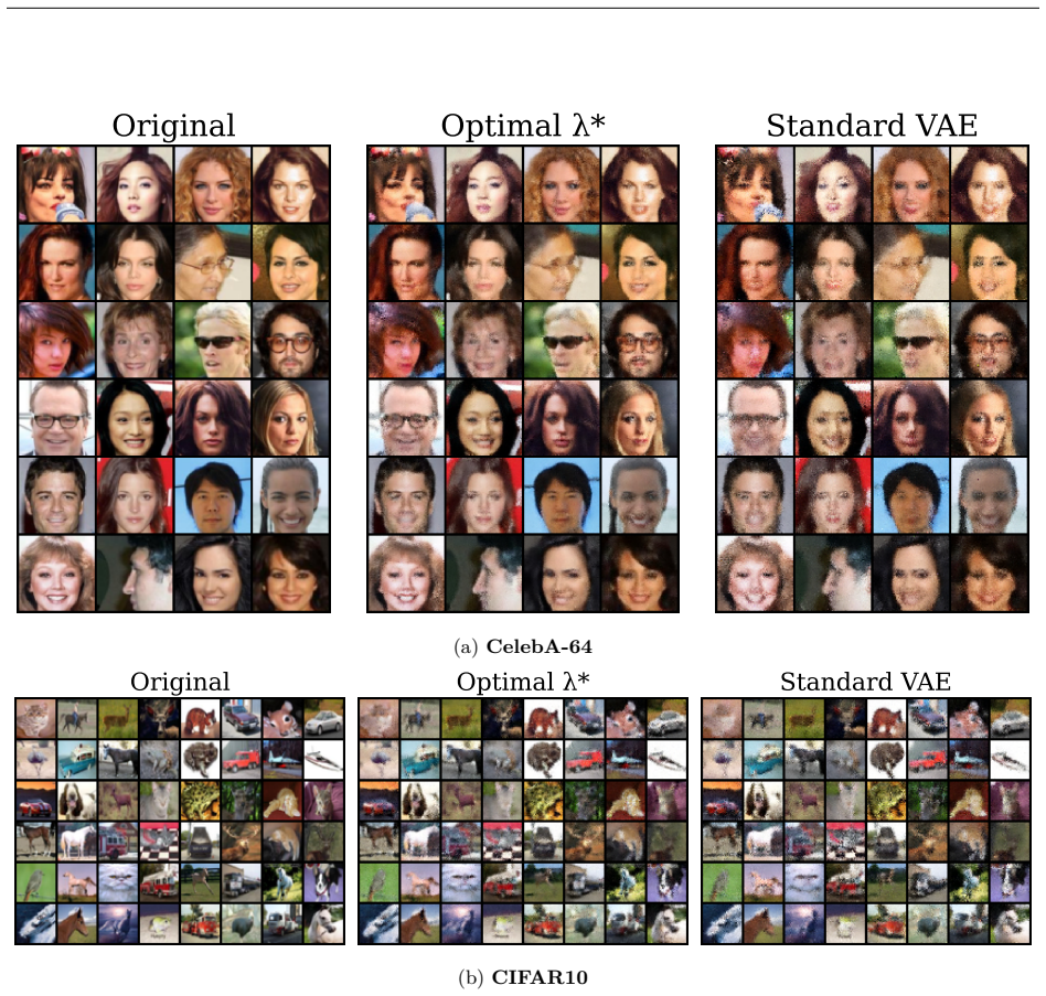

Reference graph
Works this paper leans on
-
[1]
Gener- ating sentences from a continuous space.arXiv preprint arXiv:1511.06349,
Samuel R Bowman, Luke Vilnis, Oriol Vinyals, Andrew M Dai, Rafal Jozefowicz, and Samy Bengio. Gener- ating sentences from a continuous space.arXiv preprint arXiv:1511.06349,
-
[2]
Importance weighted autoencoders.arXiv preprint arXiv:1509.00519,
Yuri Burda, Roger Grosse, and Ruslan Salakhutdinov. Importance weighted autoencoders.arXiv preprint arXiv:1509.00519,
-
[3]
Understanding disentangling in beta-vae.arXiv preprint arXiv:1804.03599,
Christopher P Burgess, Irina Higgins, Arka Pal, Loic Matthey, Nick Watters, Guillaume Desjardins, and Alexander Lerchner. Understanding disentangling in beta-vae.arXiv preprint arXiv:1804.03599,
-
[4]
Variational lossy autoencoder.arXiv preprint arXiv:1611.02731,
Xi Chen, Diederik P Kingma, Tim Salimans, Yan Duan, Prafulla Dhariwal, John Schulman, Ilya Sutskever, and Pieter Abbeel. Variational lossy autoencoder.arXiv preprint arXiv:1611.02731,
-
[5]
HaoFu, ChunyuanLi, XiaodongLiu, JianfengGao, AsliCelikyilmaz, andLawrenceCarin. Cyclicalannealing schedule: A simple approach to mitigating kl vanishing.arXiv preprint arXiv:1903.10145,
Pith/arXiv arXiv 1903
-
[6]
Accurate, large minibatch sgd: Training imagenet in 1 hour
Priya Goyal, Piotr Dollár, Ross Girshick, Pieter Noordhuis, Lukasz Wesolowski, Aapo Kyrola, Andrew Tulloch, Yangqing Jia, and Kaiming He. Accurate, large minibatch sgd: Training imagenet in 1 hour. arXiv preprint arXiv:1706.02677,
-
[7]
Pixelvae: A latent variable model for natural images.arXiv preprint arXiv:1611.05013,
Ishaan Gulrajani, Kundan Kumar, Faruk Ahmed, Adrien Ali Taiga, Francesco Visin, David Vazquez, and Aaron Courville. Pixelvae: A latent variable model for natural images.arXiv preprint arXiv:1611.05013,
-
[8]
15 Junxian He, Daniel Spokoyny, Graham Neubig, and Taylor Berg-Kirkpatrick. Lagging inference networks and posterior collapse in variational autoencoders.arXiv preprint arXiv:1901.05534,
Pith/arXiv arXiv 1901
-
[9]
Learning dynamics in linear vae: Posterior collapse threshold, su- perfluous latent space pitfalls, and speedup with kl annealing
Yuma Ichikawa and Koji Hukushima. Learning dynamics in linear vae: Posterior collapse threshold, su- perfluous latent space pitfalls, and speedup with kl annealing. InInternational Conference on Artificial Intelligence and Statistics, pp. 1936–1944. PMLR,
1936
-
[10]
Adam: A method for stochastic optimization.arXiv preprint arXiv:1412.6980,
Diederik P Kingma and Jimmy Ba. Adam: A method for stochastic optimization.arXiv preprint arXiv:1412.6980,
-
[11]
Auto-encoding variational bayes.arXiv preprint arXiv:1312.6114,
Diederik P Kingma and Max Welling. Auto-encoding variational bayes.arXiv preprint arXiv:1312.6114,
-
[12]
Adversarial autoen- coders.arXiv preprint arXiv:1511.05644,
Alireza Makhzani, Jonathon Shlens, Navdeep Jaitly, Ian Goodfellow, and Brendan Frey. Adversarial autoen- coders.arXiv preprint arXiv:1511.05644,
-
[13]
Expectation propagation for approximate bayesian inference.arXiv preprint arXiv:1301.2294,
Thomas P Minka. Expectation propagation for approximate bayesian inference.arXiv preprint arXiv:1301.2294,
-
[14]
Preventing posterior collapse with delta-vaes
16 Ali Razavi, Aäron van den Oord, Ben Poole, and Oriol Vinyals. Preventing posterior collapse with delta-vaes. arXiv preprint arXiv:1901.03416, 2019a. Ali Razavi, Aaron Van den Oord, and Oriol Vinyals. Generating diverse high-fidelity images with vq-vae-2. Advances in neural information processing systems, 32, 2019b. Danilo Rezende and Shakir Mohamed. Va...
Pith/arXiv arXiv 1901
-
[15]
Distribution matching in variational infer- ence.arXiv preprint arXiv:1802.06847,
Mihaela Rosca, Balaji Lakshminarayanan, and Shakir Mohamed. Distribution matching in variational infer- ence.arXiv preprint arXiv:1802.06847,
-
[16]
The information bottleneck method.arXiv preprint physics/0004057,
Naftali Tishby, Fernando C Pereira, and William Bialek. The information bottleneck method.arXiv preprint physics/0004057,
-
[17]
Wasserstein auto-encoders.arXiv preprint arXiv:1711.01558,
Ilya Tolstikhin, Olivier Bousquet, Sylvain Gelly, and Bernhard Schoelkopf. Wasserstein auto-encoders.arXiv preprint arXiv:1711.01558,
-
[18]
We derive the gap∆I=I(X;ϕ)−I(X;Z)≥0under Gaussian posteriors and show it attenuates change in the encoder. By theData Processing InequalityCover (1999), we have I(X;Z)≤I(X;ϕ) =⇒∆I=I(X;ϕ)−I(X;Z)≥0.(20) Sincez i =µi +σiϵi withσi >0is not invertible (givenz i =z, we cannot recoverϵi withoutµi,σi), the map is strictly lossy:∆I >0for allσi >0. Equivalently, by...
1999
discussion (0)
Sign in with ORCID, Apple, or X to comment. Anyone can read and Pith papers without signing in.