REVIEW 3 major objections 9 minor 290 references
Instanton vacuum bridges nonperturbative QCD to parton physics
Reviewed by Pith at T0; open to challenge. T0 means a machine referee read the full paper against a public rubric. the ladder, T0–T4 →
T0 review · glm-5.2
2026-07-08 17:43 UTC pith:GHLTJPCY
load-bearing objection A PhD dissertation extending the instanton liquid model to TMDs, the Collins-Soper kernel, twist-3 color-force form factors, and the nucleon EDM — broad in scope, with real new calculations but a known weak point in U(1)_A physics. the 3 major comments →
A Quantitative Framework of Nonperturbative QCD from Topological Vacuum with Application to Parton Structures
The pith
A machine-rendered reading of the paper's core claim, the machinery that carries it, and where it could break.
Core claim
The QCD instanton vacuum, parameterized solely by an instanton size of about one-third femtometer and a density of about one per cubic fermimeter, generates effective quark interactions that produce hadron spectra, form factors, parton distributions, TMDs, soft functions, and rapidity evolution kernels in a single unified framework. The same two vacuum parameters, fixed by the pion and rho masses, yield predictions for observables ranging from the Collins-Soper kernel to nucleon gravitational form factors to near-threshold J/psi photoproduction, with the author reporting consistency with lattice QCD and experiments across this range. The mechanism carrying the argument is the chirality-flip零
What carries the argument
The 't Hooft multi-fermion vertex induced by quark zero modes delocalized across the instanton ensemble; instanton-anti-instanton molecular pairs generating additional effective interactions at higher resolution; the Bethe-Salpeter equation resumming quark bubble chains to produce meson and baryon bound states; light-front projection of Bethe-Salpeter wave functions yielding partonic observables; and the grand-canonical topological ensemble connecting vacuum fluctuations to hadronic matrix elements via topological susceptibility and compressibility.
Load-bearing premise
The ILM approximates the full QCD vacuum by saturating it with instantons and anti-instantons, dropping gauge-field fluctuations that are neither self-dual nor associated with near-zero Dirac eigenmodes. If these omitted configurations contribute significantly to observables like Wilson loops, soft functions, or form factors at intermediate resolution, the framework's quantitative predictions would be systematically biased.
What would settle it
A clean falsifier would be a lattice QCD calculation showing that removing instanton-dominated configurations from gauge ensembles leaves nonperturbative observables (form factors, TMD soft functions, Collins-Soper kernel) essentially unchanged at intermediate Q^2, which would mean instantons are not the dominant carriers of nonperturbative physics the model claims them to be.
If this is right
- If the ILM parameters truly suffice to predict both hadron spectra and partonic structure, then lattice QCD calculations of PDFs, TMDs, and form factors could be cross-checked against a far cheaper semiclassical model with transparent physical interpretation.
- The nonperturbative quark-gluon operator relations derived from instanton molecules could guide targeted lattice QCD calculations by predicting which form factors are correlated and testing those correlations numerically.
- The vacuum-origin explanation of the Collins-Soper kernel, if accurate, would provide a physical mechanism for rapidity evolution that complements purely perturbative derivations and could reduce phenomenological uncertainty in TMD extractions.
- The instanton-based prediction for the nucleon electric dipole moment from strong CP offers a concrete target for next-generation neutron EDM experiments, tying a topological vacuum parameter to a potentially measurable signal.
Where Pith is reading between the lines
- The framework implicitly suggests a natural hierarchy of nonperturbative contributions: chiral-symmetry-breaking observables are dominated by isolated instantons, while confinement-sensitive and gluon-dominated observables may require the molecular or even non-self-dual configurations the ILM omits. This predicts a systematic pattern of where the model should succeed and where it should fail, whic
- The resolution-dependent splitting between dilute instantons and molecular pairs resembles a Wilsonian RG flow in topological space. One could test whether the molecular density parameter, treated as phenomenological here, can be derived from the gradient-flow evolution of lattice gauge configurations at intermediate flow times, closing the gap between the model and first-principles lattice data.
- If the two-parameter ILM genuinely captures the dominant nonperturbative physics at moderate Q^2, then the breakdown of perturbative factorization in this regime may be quantifiable as the point where instanton-induced operators compete with perturbative gluon exchange, offering a diagnostic for when pQCD-based extractions of parton distributions become unreliable.
Editorial analysis
A structured set of objections, weighed in public.
Referee Report
Summary. This dissertation develops a quantitative framework for nonperturbative QCD based on the instanton liquid model (ILM), in which the infrared QCD vacuum is modeled as an ensemble of instantons and anti-instantons. The framework is formulated both as a statistical ensemble (with weights defined by the instanton action and quark determinant) and as an effective field theory (via the 't Hooft vertex interaction). The author applies this framework to a broad range of observables: meson and baryon spectra, electromagnetic and gravitational form factors, twist-3 color Lorentz force distributions, near-threshold quarkonium photoproduction, nucleon EDM and strong CP, parton distribution functions, and transverse-momentum-dependent (TMD) soft functions including the Collins-Soper kernel. The ILM parameters (instanton size rho, density n_{I+A}, constituent mass M, molecule coupling G_IA, determinantal mass m*) are fixed primarily by the pion and rho meson masses, and the framework's predictions are compared against lattice QCD and experimental data throughout. The work demonstrates reasonable quantitative agreement (typically at the 10-30% level) across many observables, while also identifying known limitations such as the eta' mass underprediction.
Significance. The manuscript provides a comprehensive and ambitious synthesis of the instanton liquid model applied to a very wide range of hadronic observables, from spectroscopy to partonic structure. Its strengths include: (1) a unified framework connecting vacuum topology to both low-energy hadron physics and light-front parton observables; (2) explicit construction of light-front wave functions and their connection to Euclidean Bethe-Salpeter wave functions; (3) falsifiable predictions for form factors, TMD soft functions, and the Collins-Soper kernel, compared against lattice and phenomenological extractions; (4) a systematic 1/N_c and instanton-density expansion organizing the effective quark Lagrangian. The computation of the Collins-Soper kernel from the ILM (Sec. 11.4) and its comparison to recent lattice results is a particularly noteworthy new result. The framework is not parameter-free (rho, n_{I+A}, M, G_IA, m* are fitted), but the number of fitted parameters is modest relative to the range of observables addressed.
major comments (3)
- Table 4.3, eta' mass row: The ILM predicts m_{eta'} = 640 MeV versus the experimental 958 MeV, a 33% discrepancy. This is a known limitation of the N_f=2 ILM, but it is load-bearing for the central claim of 'quantitatively consistent' nonperturbative QCD. The eta' mass is set by the topological susceptibility chi_t via the Witten-Veneziano relation (Eq. 3.41), and the same chi_t enters the grand-canonical fluctuation formula (Eq. 3.149-3.152) used for hadronic matrix elements of F tilde-F, including the pseudoscalar form factor (Sec. 5.5) and nucleon EDM (Ch. 9). The manuscript should explicitly quantify the systematic uncertainty propagated from this discrepancy into observables derived from Eq. 3.149. At minimum, a clear statement is needed that the U(1)_A sector is not quantitatively controlled within the N_f=2 framework, and that observables sensitive to topological fluctuations (pse
- Sec. 3.4.5, Eq. 3.129: The determinantal mass m* is computed from the same instanton parameters (rho, n_{I+A}) that are fitted to the pion and rho masses, and m* then enters the effective 't Hooft coupling G_I in Eq. 4.2. This creates a degree of circularity in the parameter chain: rho and n_{I+A} are fixed by m_pi and m_rho; m* is derived from rho, n_{I+A}, and the quark condensate; and m* then determines G_I which feeds back into the spectrum. The manuscript should clarify which observables are genuine predictions (i.e., depend only on the fitted rho, n_{I+A}, M, and G_IA) versus those that implicitly inherit the GOR relation by construction. A flowchart or table mapping parameters to observables would strengthen the claim of quantitative consistency.
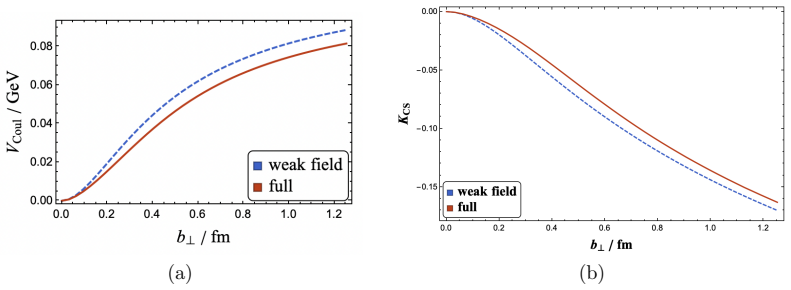
- Sec. 11.4, Eqs. 11.38 and 11.43: The Collins-Soper (CS) kernel is computed in two versions — the full ILM expression and the weak-field approximation — and compared to lattice data in Fig. 11.10. The ILM parameters used here (rho = 0.343 fm, n_{I+A} = 7.46 fm^{-4}) differ significantly from those used in the spectroscopy chapter (rho = 0.33 fm, n_{I+A} = 0.85-1.056 fm^{-4} in Tables 4.1 and 4.7). The manuscript attributes this to the dense vs. dilute ILM distinction (Sec. 3.4.3), but the prescription for choosing which parameter set applies to which observable is not systematically specified. This is load-bearing because the CS kernel result is presented as a key prediction, yet it uses a different parameter regime than the spectroscopy that fixes those parameters. A clear RG/resolution argument for the parameter choice in each chapter is needed.
minor comments (9)
- Table 4.1 caption: 'Contituent' should be 'Constituent' (also in Sec. 4.5.2 heading).
- Sec. 2.1: 'gredient flow' should be 'gradient flow' in the Chapter 3 overview (Sec. 1.1).
- Fig. 3.2 caption: 'instnaton' should be 'instanton'.
- Table 4.3: The sigma meson mass range 400-800 MeV from PDG is very broad; the ILM value of 682 MeV falls within this range, but the comparison would be more informative if the specific PDG assignment (e.g., f_0(500) vs. f_0(980)) were clarified.
- Sec. 5.6.1 and Fig. 5.21-5.22: The pion and nucleon mass decompositions are presented at two resolutions (mu ~ 1/rho and mu = 2 GeV), but the DGLAP evolution procedure used to go between them is only briefly referenced. A short statement of the evolution order (LO/NLO) and the input PDFs at the low scale would improve reproducibility.
- Sec. 9, Table 9.1: The proton and neutron EDM values are presented without uncertainties. Given the eta' mass discrepancy discussed above, an estimate of the systematic uncertainty on these predictions would be appropriate.
- Fig. 11.11 and 11.12 appear to be nearly identical plots with different captions (one referencing TMDPDFs, the other referencing the same). This may be a duplication error.
- The bibliography is extensive but several references to lattice collaborations could be updated to the most recent results (e.g., FLAG 2024 where available).
- Sec. 3.2.1, Eq. 3.28: The two-loop running is used for the instanton size distribution, but the prefactor S(ρ)^{2N_c} is only known at one-loop. The manuscript notes this but does not estimate the systematic uncertainty from the missing higher-loop prefactor.
Simulated Author's Rebuttal
We thank the referee for a careful and constructive report. The referee raises three major comments concerning: (1) the eta' mass discrepancy and its implications for observables derived from topological susceptibility, (2) the degree of circularity in the parameter chain from rho, n_{I+A} through m* to G_I, and (3) the use of different ILM parameter sets (dense vs. dilute) across chapters, particularly for the Collins-Soper kernel. We agree that all three points identify legitimate gaps in the manuscript's presentation and will revise accordingly. Below we address each comment in detail.
read point-by-point responses
-
Referee: Table 4.3, eta' mass row: The ILM predicts m_{eta'} = 640 MeV versus the experimental 958 MeV, a 33% discrepancy. This is a known limitation of the N_f=2 ILM, but it is load-bearing for the central claim of 'quantitatively consistent' nonperturbative QCD. The manuscript should explicitly quantify the systematic uncertainty propagated from this discrepancy into observables derived from Eq. 3.149. At minimum, a clear statement is needed that the U(1)_A sector is not quantitatively controlled within the N_f=2 framework, and that observables sensitive to topological fluctuations (pseudoscalar form factor, nucleon EDM) carry this systematic uncertainty.
Authors: The referee is correct that the eta' mass discrepancy is a known and significant limitation of the N_f=2 ILM, and we agree that the manuscript does not currently state this clearly enough or trace its implications for downstream observables. We will revise the manuscript to address this in three concrete ways. First, we will add an explicit statement in Sec. 4.5.3 that the U(1)_A sector is not quantitatively controlled within the N_f=2 framework: the eta' mass is underpredicted by approximately 33%, reflecting the fact that the topological susceptibility in the N_f=2 ILM is set by the instanton density and quark screening (Eq. 3.106) rather than by the full Witten-Veneziano relation with physical singlet meson masses. Second, we will add a discussion in Sec. 3.5.1 quantifying the systematic uncertainty propagated into observables derived from the grand-canonical fluctuation formula (Eqs. 3.149-3.152). The key observation is that the pseudoscalar gluonic matrix element (Eq. 3.152) is proportional to chi_t, and the ratio chi_t^{ILM}/chi_t^{WV} can be estimated from Table 3.2: the ILM prediction using exact duality gives chi_t/V = (75.1 MeV)^4 for N_f=2+1, while the Witten-Veneziano relation gives (72.6 MeV)^4, a discrepancy of approximately 4%. For the N_f=2 case used in the spectroscopy chapter, the discrepancy is larger. We will state that observables sensitive to topological fluctuations — specifically the pseudoscalar form factor (Sec. 5.5) and nucleon EDM (Ch. 9) — carry a systematic uncertainty of order this ratio, and we will add error bands or caveats to the relevant figures and tables. Third, we will clarify in the abstract and conclusion that the framework's claim of 'quantitative consistency' applies to the SU(N_f) sector and observables dominated by chiral (而非 revision: yes
-
Referee: Sec. 3.4.5, Eq. 3.129: The determinantal mass m* is computed from the same instanton parameters (rho, n_{I+A}) that are fitted to the pion and rho masses, and m* then enters the effective 't Hooft coupling G_I in Eq. 4.2. This creates a degree of circularity in the parameter chain. The manuscript should clarify which observables are genuine predictions versus those that implicitly inherit the GOR relation by construction. A flowchart or table mapping parameters to observables would strengthen the claim of quantitative consistency.
Authors: The referee identifies a legitimate concern about the parameter chain. We agree that the relationship between fitted parameters and derived quantities is not transparently presented. We will add a table (or flowchart) in Sec. 4.1 mapping the full parameter dependency structure. To be specific: the primary fitted parameters are rho, n_{I+A}, M, and G_IA, fixed by m_pi, m_rho (and m_K, m_{rho} in the N_f=3 case). The determinantal mass m* is derived from rho, n_{I+A}, and the quark condensate via Eq. 3.129, and G_I is then determined from rho, n_{I+A}, and m* via Eq. 4.2. The referee is correct that this creates a degree of circularity: observables that depend only on G_I and the GOR relation (such as the pion decay constant f_pi and the quark condensate) are not independent predictions but rather inherit the GOR relation by construction. We will explicitly classify observables into three categories: (i) fitted inputs (m_pi, m_rho, and in N_f=3 also m_K), (ii) derived quantities that inherit the GOR relation (f_pi, quark condensate, m*), and (iii) genuine predictions that depend on the fitted parameters but not on the GOR relation (e.g., meson masses other than pi and rho, baryon masses, form factors, PDFs, TMDs, CS kernel). This classification will make clear which observables test the framework independently. We note that the majority of observables presented in the dissertation — including the full meson spectrum beyond pi and rho, the baryon spectrum, all form factors in Ch. 5-9, and the partonic observables in Ch. 10-11 — fall into category (iii). revision: yes
-
Referee: Sec. 11.4, Eqs. 11.38 and 11.43: The Collins-Soper kernel uses ILM parameters (rho = 0.343 fm, n_{I+A} = 7.46 fm^{-4}) that differ significantly from those in the spectroscopy chapter (rho = 0.33 fm, n_{I+A} = 0.85-1.056 fm^{-4}). The manuscript attributes this to the dense vs. dilute ILM distinction, but the prescription for choosing which parameter set applies to which observable is not systematically specified. A clear RG/resolution argument for the parameter choice in each chapter is needed.
Authors: The referee is correct that the manuscript does not provide a systematic prescription for choosing between the dilute and dense ILM parameter sets, and that this gap undermines the presentation of the CS kernel result. We will add a clear discussion of this point. The physical basis for the distinction is the resolution scale: the dilute ILM (n_{I+A} ~ 1 fm^{-4}) corresponds to the deeply cooled regime at resolution mu ~ 1/rho ~ 600 MeV, where short-distance IA pairs have annihilated and only isolated instantons remain. The dense ILM (n_{I+A} ~ 7-10 fm^{-4}) corresponds to a higher resolution mu ~ 2 GeV, where correlated IA pairs are resolved as additional configurations (see Sec. 3.4.3 and Fig. 2.3). The key point is that the CS kernel (Sec. 11.4) and Wilson loop observables (Ch. 6) probe the vacuum at transverse distances b_perp ~ 0.1-0.3 fm, corresponding to resolution scales mu ~ 1-2 GeV, where the dense ensemble is the appropriate description. In contrast, hadron spectroscopy (Ch. 4) and form factors at low Q^2 (Ch. 5) probe the vacuum at hadronic scales ~ 1 fm, where the dilute ensemble applies. We will add a table specifying which parameter set is used in each chapter, along with the corresponding resolution scale and the physical justification. We will also add a statement in Sec. 11.4 explicitly noting that the CS kernel calculation uses the dense ILM parameters because the relevant transverse distances are shorter than the instanton separation R ~ 1 fm. We agree that without this clarification, the parameter choice appears arbitrary, and the referee's request for a systematic RG argument is well-justified. revision: yes
Circularity Check
Parameters fitted to pion/rho masses then used to 'predict' other hadron observables; GOR relation built into bosonization; η′ mass underprediction signals incomplete U(1)_A dynamics rather than circularity.
specific steps
-
fitted input called prediction
[Table 4.1 and Table 4.3 (Sec. 4.1.1, 4.5.3)]
"The fitted parameters in ILM using instanton size ρ = 0.33(2) fm and constituent mass M = 395(3) MeV with fixed pion mass mπ = 139.4 MeV and rho meson mass mρ = 785(6) MeV."
The ILM parameters (ρ, n_{I+A}, M, G_I, G_{IA}) are fixed by fitting to the physical pion and rho meson masses (Table 4.1). The Bethe-Salpeter equations (Eqs. 4.37–4.40) are then solved to produce the meson spectrum (Table 4.3). Since m_π and m_ρ are inputs to the parameter fit, their 'prediction' in Table 4.3 is tautological — the BS equation is guaranteed to reproduce them by construction of the coupling constants. The σ meson mass (682 MeV) and η′ mass (640 MeV) are genuine predictions, but the η′ underprediction by 33% indicates the framework's U(1)_A dynamics are incomplete, which is a correctness concern rather than circularity.
-
self definitional
[Eq. (4.15), Sec. 4.2 (Bosonization)]
"The last term determines the mass of the (pseudo) Goldstone boson by GOR relation. m²_π = 2mσ̄/F²_π"
The GOR relation (Eq. 4.15) is derived as a direct consequence of the bosonization procedure in Eq. (4.12). The pion mass is then used as a fitting input in Table 4.1 to fix the model parameters. When the framework subsequently 'predicts' the pion mass in Table 4.3 or uses the GOR relation to validate the chiral picture ('It successfully generate the low energy GOR relation, indicating the correct chiral picture'), this is circular: the GOR relation is built into the bosonized Lagrangian by construction, so verifying it against the same input pion mass provides no independent test.
-
fitted input called prediction
[Table 4.4, Sec. 4.5.3]
"Quark mass vs. chiral condensate in the ILM using Eqs. (4.34) and (4.35) with the parameters listed in Table 4.1 at the resolution μ = 1/ρ ≈ 600 MeV."
The current quark mass m and quark condensate ⟨q̄q⟩ are computed from the gap equations (4.34, 4.35) using the parameters already fitted to m_π and m_ρ in Table 4.1. Since the GOR relation m²_π = 2m⟨q̄q⟩/F²_π is built into the framework (Eq. 4.15), the product m|⟨q̄q⟩| is constrained to match the pion mass input by construction. The comparison to FLAG lattice values in Table 4.4 is therefore not an independent prediction but a consistency check of the fitted parameters against the same GOR relation that lattice QCD also satisfies.
full rationale
The paper fits ILM parameters (ρ, n_{I+A}, M, G_I, G_{IA}) to the physical pion and rho meson masses (Table 4.1), then uses the Bethe-Salpeter equation to produce a meson spectrum (Table 4.3) where m_π and m_ρ are reproduced by construction. The GOR relation is built into the bosonization procedure (Eq. 4.15), so the quark mass and condensate in Table 4.4 are constrained by the pion mass input. However, the framework does produce genuinely independent predictions for observables not used in fitting: the σ meson mass, gravitational form factors (Ch. 5), TMD soft functions (Ch. 11), color force form factors (Ch. 8), and EDM (Ch. 9) are computed from the same parameters but are not fitted. The η′ mass underprediction (640 vs 958 MeV) is a correctness limitation of the ILM's U(1)_A dynamics, not a circularity issue. Self-citations to prior ILM work (Refs. [30, 31, 32, 33, 34, 35, 36, 37, 38, 39, 40, 41]) are used to reference established methodology, not to import unverified uniqueness theorems. The circularity is moderate: the central spectroscopic results are partially constrained by the fit, but the broader framework's applications to form factors, PDFs, and TMDs contain substantial independent content.
Axiom & Free-Parameter Ledger
free parameters (9)
- rho (instanton size) =
0.33(2) fm
- n_I+A (instanton density) =
~0.85-1.0 fm^-4
- M (constituent quark mass) =
395(3) MeV
- G_IA (molecule coupling) =
67.8 GeV^-2 (Nf=2), 64.8 GeV^-2 (Nf=3)
- m* (determinantal mass) =
~103.6 MeV
- n_mol (molecule density) =
7.248 fm^-4
- m_0++ (scalar glueball mass) =
1.5-1.7 GeV
- sigma_piN (pion-nucleon sigma term) =
45-60 MeV
- m_3g (three-gluon exchange mass) =
1.49 GeV
axioms (6)
- domain assumption QCD vacuum is saturated by instantons and anti-instantons at low resolution
- domain assumption Large-Nc planar resummation captures dominant quark dynamics in instanton vacuum
- ad hoc to paper Instanton size distribution is sharply peaked at mean value rho
- domain assumption Two-body semiclassical interactions suffice for instanton ensemble
- domain assumption Zero-mode dominance for light quarks in instanton background
- ad hoc to paper Ratio ansatz for IA pair interaction
invented entities (2)
-
Instanton-anti-instanton molecules (dense ILM)
independent evidence
-
Determinantal mass m*
independent evidence
read the original abstract
This dissertation develops a quantitative framework that provides a physical picture for non-perturbative QCD based on the topological structure of the QCD vacuum. By integrating out the ultraviolet degrees of freedom, the infrared gluon configurations are modeled as a liquid ensemble of instantons and anti-instantons, which induce effective interactions among quarks. This framework captures the origin of trace and axial anomalies through the infrared distributions of QCD and dynamically breaks chiral symmetry. More specifically, this framework can be formulated in two ways: in one, we construct a statistical ensemble with weights defined by the instanton action and Dirac determinant, while in the other we formulate an effective field theory (EFT) by rewriting the determinant as effective quark interactions. By reformulating the EFT on the light front, we explicitly construct the light-front wave functions and calculate various parton observables in linear factorization. We further embed the framework into transverse momentum dependent factorization and establish a vacuum origin for rapidity evolution by computing the soft functions. We also extend this approach to various form factors in light hadrons, including scalar, pseudoscalar, and energy-momentum tensor (EMT), as well as higher-twist color force and multigluon correlations, with applications to hadron mass and spin decomposition, near-threshold quarkonium production, and strong CP problem, highlighting the importance of the vacuum origin in hadron structures. Overall, this work demonstrates that the QCD vacuum provides a quantitatively crucial description of hadronic structure from low to moderate resolution, bridging nonperturbative vacuum physics with partonic phenomenology.
Figures































Reference graph
Works this paper leans on
-
[1]
Magnetic Monopoles in Unified Gauge Theories.Nucl
Gerard ’t Hooft. Magnetic Monopoles in Unified Gauge Theories.Nucl. Phys. B, 79:276–284, 1974. doi: 10.1016/0550-3213(74)90486-6
- [2]
-
[3]
A. A. Belavin, Alexander M. Polyakov, A. S. Schwartz, and Yu. S. Tyupkin. Pseudoparticle Solutions of the Yang-Mills Equations.Phys. Lett. B, 59:85–87, 1975. doi: 10.1016/0370-2693(75)90163-X
-
[4]
Thomas C. Kraan and Pierre van Baal. Monopole constituents inside SU(n) calorons.Phys. Lett. B, 435:389–395, 1998. doi: 10.1016/ S0370-2693(98)00799-0
work page 1998
-
[5]
Dmitri Diakonov and V. Yu. Petrov. Instanton Based Vacuum from Feynman Variational Principle.Nucl. Phys. B, 245:259–292, 1984. doi: 10.1016/0550-3213(84)90432-2
-
[6]
Curtis G. Callan, Jr., R. F. Dashen, and David J. Gross. The Structure of the Gauge Theory Vacuum.Phys. Lett. B, 63:334–340, 1976. doi: 10.1016/0370-2693(76)90277-X
-
[7]
Curtis G. Callan, Jr., Roger F. Dashen, and David J. Gross. Toward a Theory of the Strong Interactions.Phys. Rev. D, 17:2717, 1978. doi: 10.1103/PhysRevD.17.2717
-
[8]
Edward V. Shuryak. The Role of Instantons in Quantum Chromo- dynamics. 1. Physical Vacuum.Nucl. Phys. B, 203:93, 1982. doi: 10.1016/0550-3213(82)90478-3
-
[9]
Dmitri Diakonov and V. Yu. Petrov. A Theory of Light Quarks in the Instanton Vacuum.Nucl. Phys. B, 272:457–489, 1986. doi: 10.1016/ 0550-3213(86)90011-8. 276
work page 1986
-
[10]
A. I. Vainshtein, Valentin I. Zakharov, V. A. Novikov, and Mikhail A. Shifman. ABC’s of Instantons.Sov. Phys. Usp., 25:195, 1982. doi: 10.1070/PU1982v025n04ABEH004533
-
[11]
Chiral symmetry breaking by instantons
Dmitri Diakonov. Chiral symmetry breaking by instantons. Proc. Int. Sch. Phys. Fermi, 130:397–432, 1996. doi: 10.3254/ 978-1-61499-215-8-397
work page 1996
-
[12]
Hadronic structure on the light-front
Nicholas Miesch, Edward Shuryak, and Ismail Zahed. Hadronic structure on the light-front. IX. Orbital-spin-isospin wave functions of baryons. Phys. Rev. D, 108(9):094033, 2023. doi: 10.1103/PhysRevD.108.094033
-
[13]
Hadronic structure on the light front
Edward Shuryak and Ismail Zahed. Hadronic structure on the light front. V. Diquarks, nucleons, and multiquark Fock components.Phys. Rev. D, 107(3):034027, 2023. doi: 10.1103/PhysRevD.107.034027
-
[14]
Hadronic structure on the light front
Edward Shuryak and Ismail Zahed. Hadronic structure on the light front. IV. Heavy and light baryons.Phys. Rev. D, 107(3):034026, 2023. doi: 10.1103/PhysRevD.107.034026
-
[15]
How Instantons Solve the U(1) Problem.Phys
Gerard ’t Hooft. How Instantons Solve the U(1) Problem.Phys. Rept., 142:357–387, 1986. doi: 10.1016/0370-1573(86)90117-1
-
[16]
The Hadron-Parton Bridge, From the QCD Vacuum to Partons
Edward Shuryak and Ismail Zahed. The Hadron-Parton Bridge, From the QCD Vacuum to Partons. 1 2026
work page 2026
-
[17]
Edward Shuryak.Nonperturbative Topological Phenomena in QCD and Related Theories. Springer Cham, March 2021. doi: 10.1007/ 978-3-030-62990-8
work page 2021
-
[18]
Thomas Sch¨ afer and Edward V. Shuryak. Instantons in QCD.Rev. Mod. Phys., 70:323–426, 1998. doi: 10.1103/RevModPhys.70.323
-
[19]
Christopher Michael and P. S. Spencer. Instanton size distributions from calibrated cooling.Nucl. Phys. B Proc. Suppl., 42:261–263, 1995. doi: 10.1016/0920-5632(95)00220-4
-
[20]
Christopher Michael and P. S. Spencer. Cooling and the SU(2) instanton vacuum.Phys. Rev. D, 52:4691–4699, 1995. doi: 10.1103/PhysRevD.52. 4691
- [21]
-
[22]
Gradient flows and instantons at a Lifshitz point.J
Ioannis Bakas. Gradient flows and instantons at a Lifshitz point.J. Phys. Conf. Ser., 283:012004, 2011. doi: 10.1088/1742-6596/283/1/012004
-
[23]
Biddle, Waseem Kamleh, and Derek B
James C. Biddle, Waseem Kamleh, and Derek B. Leinweber. Visualizations of Centre Vortex Structure in Lattice Simulations.PoS, LATTICE2018:256, 2018. doi: 10.22323/1.334.0256
-
[24]
Continuous renormalization group βfunction from lattice simulations.Phys
Anna Hasenfratz and Oliver Witzel. Continuous renormalization group βfunction from lattice simulations.Phys. Rev. D, 101(3):034514, 2020. doi: 10.1103/PhysRevD.101.034514
-
[25]
A. Athenodorou, Ph. Boucaud, F. De Soto, J. Rodr´ ıguez-Quintero, and S. Zafeiropoulos. Instanton liquid properties from lattice QCD.JHEP, 02:140, 2018. doi: 10.1007/JHEP02(2018)140
-
[26]
Biddle, Waseem Kamleh, and Derek B
James C. Biddle, Waseem Kamleh, and Derek B. Leinweber. Visualisations of Centre Vortices.EPJ Web Conf., 245:06010, 2020. doi: 10.1051/epjconf/202024506010
-
[27]
Extracting Instantons from the Lattice.PoS, LATTICE2023:376, 2024
Falk Zimmermann. Extracting Instantons from the Lattice.PoS, LATTICE2023:376, 2024. doi: 10.22323/1.453.0376
-
[28]
A. Ringwald and F. Schrempp. Confronting instanton perturbation theory with QCD lattice results.Phys. Lett. B, 459:249–258, 1999. doi: 10.1016/S0370-2693(99)00682-6
-
[29]
Pietro Faccioli and Thomas A. DeGrand. Evidence for instanton induced dynamics, from lattice QCD.Phys. Rev. Lett., 91:182001, 2003. doi: 10.1103/PhysRevLett.91.182001
-
[30]
Glue in hadrons at medium resolution and the QCD instanton vacuum.Phys
Wei-Yang Liu, Edward Shuryak, and Ismail Zahed. Glue in hadrons at medium resolution and the QCD instanton vacuum.Phys. Rev. D, 110 (5):054005, 2024. doi: 10.1103/PhysRevD.110.054005
-
[31]
Generic framework for non-perturbative QCD in light hadrons
Wei-Yang Liu. Generic framework for non-perturbative QCD in light hadrons. 1 2025
work page 2025
-
[32]
Hadronic structure on the light-front
Wei-Yang Liu, Edward Shuryak, and Ismail Zahed. Hadronic structure on the light-front. VII. Pions and kaons and their partonic distributions. Phys. Rev. D, 107(9):094024, 2023. doi: 10.1103/PhysRevD.107.094024
-
[33]
Hadronic structure on the light front
Wei-Yang Liu, Edward Shuryak, and Ismail Zahed. Hadronic structure on the light front. VIII. Light scalar and vector mesons.Phys. Rev. D, 109(7):074029, 2024. doi: 10.1103/PhysRevD.109.074029. 278
-
[34]
Pion gravitational form factors in the QCD instanton vacuum
Wei-Yang Liu, Edward Shuryak, Christian Weiss, and Ismail Zahed. Pion gravitational form factors in the QCD instanton vacuum. I.Phys. Rev. D, 110(5):054021, 2024. doi: 10.1103/PhysRevD.110.054021
-
[35]
Pion gravitational form factors in the QCD instanton vacuum
Wei-Yang Liu, Edward Shuryak, and Ismail Zahed. Pion gravitational form factors in the QCD instanton vacuum. II.Phys. Rev. D, 110(5): 054022, 2024. doi: 10.1103/PhysRevD.110.054022
-
[36]
Collins-Soper Kernel in the QCD Instanton Vacuum
Wei-Yang Liu, Ismail Zahed, and Yong Zhao. Collins-Soper Kernel in the QCD Instanton Vacuum. 12 2024
work page 2024
-
[37]
Photoproduction ofηc,b near threshold
Wei-Yang Liu and Ismail Zahed. Photoproduction ofηc,b near threshold. Phys. Rev. D, 110(5):054025, 2024. doi: 10.1103/PhysRevD.110.054025
-
[38]
The color force acting on a quark in the pion and nucleon
Wei-Yang Liu, Edward Shuryak, and Ismail Zahed. The color force acting on a quark in the pion and nucleon. 11 2025
work page 2025
-
[39]
Nucleon electric dipole form factor in QCD vacuum
Wei-Yang Liu and Ismail Zahed. Nucleon electric dipole form factor in QCD vacuum. 1 2025
work page 2025
-
[40]
Wei-Yang Liu and Ismail Zahed. Tomography of pions and kaons in the QCD vacuum: Transverse momentum dependent parton distribution functions.Phys. Rev. D, 112(3):034039, 2025. doi: 10.1103/9t4h-zpwm
-
[41]
Wei-Yang Liu and Ismail Zahed. Tomography of the rho meson in the QCD instanton vacuum: Transverse momentum dependent parton distribution functions.Phys. Rev. D, 112(3):034028, 2025. doi: 10.1103/ 6ffp-qs8p
work page 2025
-
[42]
Trivializing maps, the Wilson flow and the HMC algorithm.Commun
Martin Luscher. Trivializing maps, the Wilson flow and the HMC algorithm.Commun. Math. Phys., 293:899–919, 2010. doi: 10.1007/ s00220-009-0953-7
work page 2010
-
[43]
Perturbative analysis of the gradient flow in non-abelian gauge theories.JHEP, 02:051, 2011
Martin Luscher and Peter Weisz. Perturbative analysis of the gradient flow in non-abelian gauge theories.JHEP, 02:051, 2011. doi: 10.1007/ JHEP02(2011)051
work page 2011
-
[44]
Future applications of the Yang-Mills gradient flow in lattice QCD.PoS, LATTICE2013:016, 2014
Martin L¨ uscher. Future applications of the Yang-Mills gradient flow in lattice QCD.PoS, LATTICE2013:016, 2014. doi: 10.22323/1.187.0016
-
[45]
Gradient flow and the Wilsonian renormalization group flow.PTEP, 2018(5):053B02, 2018
Hiroki Makino, Okuto Morikawa, and Hiroshi Suzuki. Gradient flow and the Wilsonian renormalization group flow.PTEP, 2018(5):053B02, 2018. doi: 10.1093/ptep/pty050. 279
-
[46]
R. Narayanan and H. Neuberger. Infinite N phase transitions in continuum Wilson loop operators.JHEP, 03:064, 2006. doi: 10.1088/ 1126-6708/2006/03/064
work page 2006
-
[47]
P. J. Moran and D. B. Leinweber. Buried treasure in the sand of the QCD vacuum. InQCD Downunder II, 5 2008
work page 2008
-
[48]
Gluons, light and heavy quarks and their interactions in the instanton vacuum
Mirzayusuf Musakhanov. Gluons, light and heavy quarks and their interactions in the instanton vacuum. 3 2023
work page 2023
-
[49]
Instantons in qcd: Theory and application of the instanton liquid model, 2001
Marcus Hutter. Instantons in qcd: Theory and application of the instanton liquid model, 2001. URLhttps://arxiv.org/abs/hep-ph/ 0107098
work page 2001
-
[50]
Rapp, Thomas Sch¨ afer, Edward V
R. Rapp, Thomas Sch¨ afer, Edward V. Shuryak, and M. Velkovsky. Diquark Bose condensates in high density matter and instantons.Phys. Rev. Lett., 81:53–56, 1998. doi: 10.1103/PhysRevLett.81.53
-
[51]
Rapp, Thomas Sch¨ afer, Edward V
R. Rapp, Thomas Sch¨ afer, Edward V. Shuryak, and M. Velkovsky. High density QCD and instantons.Annals Phys., 280:35–99, 2000. doi: 10. 1006/aphy.1999.5991
-
[52]
Ernst-Michael Ilgenfritz and Edward V. Shuryak. Chiral Symmetry Restoration at Finite Temperature in the Instanton Liquid.Nucl. Phys. B, 319:511–520, 1989. doi: 10.1016/0550-3213(89)90617-2
-
[53]
Hadronic structure on the light front
Edward Shuryak and Ismail Zahed. Hadronic structure on the light front. I. Instanton effects and quark-antiquark effective potentials.Phys. Rev. D, 107(3):034023, 2023. doi: 10.1103/PhysRevD.107.034023
-
[54]
Edward V. Shuryak. Toward the Quantitative Theory of the ’Instanton Liquid’ 4. Tunneling in the Double Well Potential.Nucl. Phys. B, 302: 621–644, 1988. doi: 10.1016/0550-3213(88)90191-5
-
[55]
I. I. Balitsky and A. V. Yung. Collective - Coordinate Method for Quasizero Modes.Phys. Lett. B, 168:113–119, 1986. doi: 10.1016/ 0370-2693(86)91471-1
work page 1986
-
[56]
A. V. Yung. Instanton Vacuum in Supersymmetric QCD.Nucl. Phys. B, 297:47, 1988. doi: 10.1016/0550-3213(88)90199-X
-
[57]
J. J. M. Verbaarschot. Streamlines and conformal invariance in Yang- Mills theories.Nucl. Phys. B, 362:33–53, 1991. doi: 10.1016/ 0550-3213(91)90554-B. [Erratum: Nucl.Phys.B 386, 236–236 (1992)]. 280
work page 1991
-
[58]
D. M. Ostrovsky, G. W. Carter, and E. V. Shuryak. Forced tunneling and turning state explosion in pure Yang-Mills theory.Phys. Rev., D66: 036004, 2002. doi: 10.1103/PhysRevD.66.036004
-
[59]
Frans R. Klinkhamer and N. S. Manton. A Saddle Point Solution in the Weinberg-Salam Theory.Phys. Rev., D30:2212, 1984. doi: 10.1103/ PhysRevD.30.2212
work page 1984
-
[60]
How to observe the QCD instanton/sphaleron processes at hadron colliders? 1 2021
Edward Shuryak and Ismail Zahed. How to observe the QCD instanton/sphaleron processes at hadron colliders? 1 2021
work page 2021
-
[61]
Michael F. Atiyah and Isadore M. Singer. The index of elliptic operators on compact manifolds.Bulletin of the American Mathematical Society, 69:322–433, 1963. doi: 10.1090/S0002-9904-1963-10957-X
-
[62]
Confinement from Center Vortices: A review of old and new results.EPJ Web Conf., 137:01009, 2017
Jeff Greensite. Confinement from Center Vortices: A review of old and new results.EPJ Web Conf., 137:01009, 2017. doi: 10.1051/epjconf/ 201713701009
-
[63]
Potential energy of Yang-Mills vortices in three- dimensions and four-dimensions.Mod
Dmitri Diakonov. Potential energy of Yang-Mills vortices in three- dimensions and four-dimensions.Mod. Phys. Lett. A, 14:1725–1732,
-
[64]
doi: 10.1142/S0217732399001826
-
[65]
Center vortex solutions of the Yang- Mills effective action in three and four dimensions.Phys
Dmitri Diakonov and Martin Maul. Center vortex solutions of the Yang- Mills effective action in three and four dimensions.Phys. Rev. D, 66: 096004, 2002. doi: 10.1103/PhysRevD.66.096004
-
[66]
On the spectrum of the Faddeev-Popov operator in topological background fields.Eur
Axel Maas. On the spectrum of the Faddeev-Popov operator in topological background fields.Eur. Phys. J. C, 48:179–192, 2006. doi: 10.1140/epjc/s10052-006-0003-y
-
[67]
Biddle, Waseem Kamleh, and Derek B
James C. Biddle, Waseem Kamleh, and Derek B. Leinweber. Visualization of center vortex structure.Phys. Rev. D, 102(3):034504,
-
[68]
doi: 10.1103/PhysRevD.102.034504
-
[69]
K. Langfeld, O. Tennert, M. Engelhardt, and H. Reinhardt. Center vortices of Yang-Mills theory at finite temperatures.Phys. Lett. B, 452: 301, 1999. doi: 10.1016/S0370-2693(99)00252-X
-
[70]
Waseem Kamleh, Derek B. Leinweber, and Adam Virgili. Numerical indication that center vortices drive dynamical mass generation in QCD. Phys. Rev. D, 110(5):L051502, 2024. doi: 10.1103/PhysRevD.110. L051502. 281
-
[71]
Mendel Nguyen, Tin Sulejmanpasic, and Mithat ¨Unsal. Phases of Theories with ZN 1-Form Symmetry, and the Roles of Center Vortices and Magnetic Monopoles.Phys. Rev. Lett., 134(14):141902, 2025. doi: 10.1103/PhysRevLett.134.141902
-
[72]
Self-dual monopole loops, instantons and confinement
Mendel Nguyen and Mithat ¨Unsal. Self-dual monopole loops, instantons and confinement. 9 2025
work page 2025
-
[73]
Unifying Monopole and Center Vortex as the Semiclassical Confinement Mechanism.Phys
Yui Hayashi and Yuya Tanizaki. Unifying Monopole and Center Vortex as the Semiclassical Confinement Mechanism.Phys. Rev. Lett., 133(17): 171902, 2024. doi: 10.1103/PhysRevLett.133.171902
-
[74]
Canberk G¨ uvendik, Thomas Schaefer, and Mithat ¨Unsal. The metamorphosis of semi-classical mechanisms of confinement: from monopoles onR 3 ×S 1 to center-vortices onR 2 ×T 2.JHEP, 11:163,
-
[75]
doi: 10.1007/JHEP11(2024)163
-
[76]
Thomas C. Kraan and Pierre van Baal. Periodic instantons with nontrivial holonomy.Nucl. Phys. B, 533:627–659, 1998. doi: 10.1016/ S0550-3213(98)00590-2
work page 1998
-
[78]
Thomas C. Kraan and Pierre van Baal. Exact T duality between calorons and Taub - NUT spaces.Phys. Lett. B, 428:268–276, 1998. doi: 10.1016/ S0370-2693(98)00411-0
work page 1998
-
[79]
Ariel R. Zhitnitsky. Confinement- deconfinement phase transition and fractional instanton quarks in dense matter. InLight-Cone QCD and Nonperturbative Hadron Physics, pages 207–213, 1 2006. doi: 10.1142/ 9789812708267 0023
work page 2006
-
[80]
Mithat Unsal and Laurence G. Yaffe. Center-stabilized Yang-Mills theory: Confinement and large N volume independence.Phys. Rev. D, 78:065035, 2008. doi: 10.1103/PhysRevD.78.065035
-
[81]
Light quarks in the screened dyon-antidyon Coulomb liquid model
Yizhuang Liu, Edward Shuryak, and Ismail Zahed. Light quarks in the screened dyon-antidyon Coulomb liquid model. II.Phys. Rev. D, 92(8): 085007, 2015. doi: 10.1103/PhysRevD.92.085007
discussion (0)
Sign in with ORCID, Apple, or X to comment. Anyone can read and Pith papers without signing in.