REVIEW 3 major objections 5 minor 46 references
Machine learning finds structured predictability in bias-corrected supernova residuals that look closed in redshift bins.
Reviewed by Pith at T0; open to challenge. T0 means a machine referee read the full paper against a public rubric. the ladder, T0–T4 →
Out-of-fold LightGBM recovers up to R²=0.982 of bias-corrected Hubble residual variance in LSST SN Ia mocks and R²=0.725 on DES 5YR, with consistent SHAP rankings, while redshift bins explain <1%.
T0 review reviewed 2026-07-10 challenge →
load-bearing objection Solid methods paper: a reusable residual-predictability scorecard that catches multivariate structure redshift bins miss, with the arithmetic-baseline issue already handled carefully enough that the diagnostic still stands. the 3 major comments →
Machine Learning Closure Audits for LSST Photometric Supernova Cosmology
The pith
A machine-rendered reading of the paper's core claim, the machinery that carries it, and where it could break.
The reading
Core claim
Bias-corrected Hubble residuals that appear closed under redshift-binned means retain strong multivariate predictability: out-of-fold LightGBM models reach R² up to 0.982 on the M25 LSST-like simulation and 0.945–0.979 on M23 mocks (versus R²_z < 0.01), and the same audit on DES 5YR spectroscopic SNe Ia yields held-out R² = 0.725, with independent M25 and DES shared-feature SHAP rankings agreeing at Spearman ρ = 0.802.
What carries the argument
Supervised ML closure audit: train held-out LightGBM (and ablation baselines) to predict bias-corrected residual Δμ from measured observables, then score with out-of-fold R²/RMSE plus SHAP attributions and a reusable scorecard that compares mock ensembles to real data.
Load-bearing premise
That residual predictability beyond the four core light-curve and redshift variables is a meaningful non-closure signal, not mostly arithmetic reconstruction of a residual that is already built from those same fitted quantities.
What would settle it
On a matched mock ensemble and real sample with identical feature inventories, find that held-out R² remains near the redshift-bin baseline (≪0.1) and that SHAP rankings do not agree across simulation and real data, or that full-model gains vanish once core Tripp variables and analysis-stage outputs are removed.
Editorial analysis
A structured set of objections, weighed in public.
Referee Report
Summary. The paper proposes a supervised machine-learning closure audit for simulation-dependent SN Ia cosmology pipelines. After standard light-curve fitting and BBC-style bias corrections, it trains held-out LightGBM (and comparison) models to predict the bias-corrected Hubble residual Δμ from measured observables, reporting R² and RMSE plus SHAP attributions. On M23 and M25 LSST-like mocks, redshift-binned means give R²_z < 0.01 while full models reach R² up to 0.982; a four-feature Tripp core {x1, c, mB, zHD} already yields R²_core = 0.791–0.957, with modest incremental gains ΔR². The same shared-feature audit on DES 5YR spectroscopic SNe Ia gives held-out R² = 0.725, and M25/DES SHAP rankings agree at Spearman ρ = 0.802. Feature ablations, fold-stable rankings, 19 FITOPT systematics, and an Appendix C stress test against using the ML model as a direct cosmological correction support a reusable scorecard intended as a pre-unblinding diagnostic, not a distance estimator.
Significance. If the incremental residual structure beyond arithmetic reconstruction of Δμ is scientifically meaningful, the work supplies a practical, reusable diagnostic layer for LSST-scale photometric SN cosmology that standard one-dimensional redshift summaries miss. Strengths include realisation-held-out five-fold CV, multi-algorithm checks (LightGBM, ExtraTrees, Ridge), feature-family ablations, fold-stable SHAP rankings (⟨ρ⟩ = 0.990), robustness across 19 systematic variants, an independent real-data DES application, and an explicit Appendix C demonstration that direct ML residual correction is cosmology-dependent and unsafe. The scorecard template (Table 6) and shared-feature M25–DES comparison are concrete deliverables that other pipelines can adopt.
major comments (3)
- [§3.1–3.2, Eq. (2), Table 2] Sections 3.1–3.2 and Eq. (2): the central interpretive claim is that residual predictability is a non-closure diagnostic. Because Δμ is constructed from mB, x1, c, z and bias terms, R²_core is largely arithmetic by design; the paper correctly flags this but still leads with absolute R² = 0.982 (abstract, Table 2, §4.2). For M25 the incremental gain is only ΔR² = 0.024. The manuscript should re-centre the scorecard and abstract on ΔR², null baselines, and non-Tripp structure, and state more clearly what absolute R² alone does and does not mean for closure.
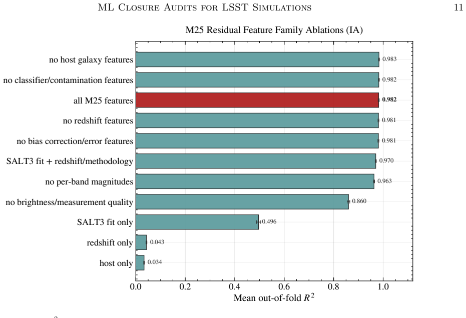
- [§4.4, Table 4, Fig. 2] §4.4 and Table 4 / Fig. 2: ablations show that removing the brightness/measurement-quality family drops R² from 0.982 to 0.860, while host-only and bias-only models are weak, yet top SHAP features include Y/z-band magnitudes (strongly correlated with mB and zHD) and analysis-stage outputs (biasCor_mu, MUERR_RENORM, etc.). A stricter leakage control—e.g., a model that excludes all quantities that enter or tightly proxy Eq. (2) and the BBC grid, or an explicit residual-after-Tripp-reconstruction target—is needed to show how much of the remaining signal is selection/dust/host physics rather than correlated photometry and pipeline outputs.
- [Table 6, §5, Appendix C] Table 6 and §5: operational flags (R² ≥ 0.10, ΔR² ≥ 0.05, >2σ_mock) are proposed as starting points, but Appendix C only shows that direct ML correction is unsafe; it does not map scorecard metrics onto bias in w0 or Ωm for the actual M23/M25 residual field. Without that mapping, or a clear statement that thresholds remain uncalibrated for cosmology impact, the claim that the scorecard identifies residual non-closure before unblinding overstates the current quantitative link to cosmological parameters.
minor comments (5)
- [Table 1, §4.1] Table 1 note correctly warns that M23/M25 differ in many simultaneous ways; the main text still sometimes reads as a progressive sequence. Soften comparative language in §4.1.
- [Fig. 3] Figure 3 caption and text should state more prominently that the map is an observed-manifold summary of held-out predictions, not a causal partial-dependence or marginalised host-step measurement.
- [§4.5] DES shared-feature set omits DES griz magnitudes for matching; a short DES-only full-feature audit (even if not compared to M25) would strengthen the real-data claim in §4.5.
- [Abstract, Eq. (1)–(2)] Minor typos and notation: abstract/body capitalisation of Redshift; R 2 spacing; occasional Δμ vs Δμ notation inconsistency; ensure Eq. (1)–(2) symbols match the text.
- [Appendix A] Appendix A inventories are valuable; a one-line statement of how many columns were dropped for leakage/missingness would aid reproducibility.
Circularity Check
Partial self-definitional circularity: high R² on Δμ is driven largely by arithmetic reconstruction from the Tripp parameters that define it (Eq. 2), which the paper flags as baseline R²_core but still presents absolute predictability as the main non-closure signal.
specific steps
-
self definitional
[Eq. 2; Sections 3.1–3.2, 4.2]
"Δμ=m B +αx 1 −βc+M 0 + Δμbias −μ model(z) ... Because the target residual Δμ is mathematically constructed from fitted light curve parameters and redshift (Equation 2), the Tripp set model has an expected arithmetic component. We therefore treat its performance, R 2 core, as an arithmetic baseline ... high predictability can arise partly because Δμ is constructed from fitted light curve and redshift parameters"
The target residual is defined directly from the core predictors {mB, x1, c, z} plus bias and model terms. Predicting Δμ from those same quantities (R²_core = 0.791–0.957) is therefore largely arithmetic reconstruction by construction, not an independent discovery of residual structure. The paper correctly demotes R²_core to a baseline and reports ΔR², yet still leads with absolute full-model R² (0.945–0.982) as evidence of non-closure that 1-D tests miss; most of that absolute figure is the definitional component plus correlated photometric proxies.
-
fitted input called prediction
[Section 4.2–4.4; Table 3; Figure 2/5]
"Relative to the four feature Tripp standardisation model (R 2 = 0.957), the full audit gains ΔR2 = 0.024 ... Removing the full [brightness and measurement quality] family drops R 2 from 0.982 to 0.860 ... Yband peak magnitude is strongly correlated with the fitted apparent magnitude mB (r= 0.993)"
Band magnitudes, SNRs and analysis-stage outputs (biasCor_mu, MUERR, etc.) that dominate SHAP and ablations are either direct inputs to Δμ or extremely tight empirical proxies for the defining terms. The incremental ΔR² and “brightness/measurement quality” signal therefore partly re-expresses the same arithmetic construction under different labels rather than isolating purely external residual physics. The paper’s own ablations and correlation checks make this reduction visible.
full rationale
The paper’s central diagnostic is that out-of-fold models recover high residual variance (R² up to 0.982) while redshift-binned means give R²_z < 0.01, revealing structured non-closure. Equation 2 defines the target as Δμ = mB + α x1 − β c + M0 + Δμ_bias − μ_model(z), so the four-feature Tripp core is definitionally related to the target; the paper itself labels R²_core an “arithmetic baseline” and focuses on ΔR² and non-core features. That acknowledgment prevents full circularity, and independent content remains (DES held-out R² = 0.725, M25–DES SHAP Spearman ρ = 0.802, brightness/SNR ablations, systematic robustness). Absolute high R² values and the claim of “structured residual predictability” nevertheless rest partly on reconstruction of quantities that enter the residual by construction, plus tightly correlated proxies (band magnitudes r ≈ 0.99 with mB). No load-bearing uniqueness theorem or self-citation chain forces the result; the circularity is limited to the definitional component of the predictability metric. Score 4 reflects partial reduction by construction with remaining independent diagnostic content.
Axiom & Free-Parameter Ledger
free parameters (4)
- LightGBM baseline hyperparameters =
N_trees=1000, lr=0.05, N_leaves=63
- Operational non-closure thresholds (Table 6) =
R²≥0.10; ΔR²≥0.05; >2σ_mock
- Host-mass split for manifold map =
10
- Redshift bin count for null baseline =
6 bins
axioms (5)
- domain assumption Bias-corrected Hubble residual Δμ is the appropriate target for a closure audit and should be featureless after standard BBC/SALT processing.
- ad hoc to paper Held-out R² and RMSE on measured observables are valid diagnostics of residual non-closure even though Δμ is constructed from light-curve and redshift parameters (Eq. 2).
- domain assumption M23/M25 mock realisations and DES 5YR spectroscopic sample are sufficiently representative for the audit comparison.
- standard math SHAP mean absolute values rank predictive contribution without implying physical causation.
- domain assumption Simulation held-out five-fold splits by realisation eliminate train–test leakage.
invented entities (1)
-
ML closure audit scorecard (Table 2 / Table 6 template)
no independent evidence
Cite this review
Pith. "Pith review of Machine Learning Closure Audits for LSST Photometric Supernova Cosmology." pith.science (2026). https://pith.science/paper/TKD347WX
@misc{pith2026260706734,
  author       = {Pith},
  title        = {Pith review of: Machine Learning Closure Audits for LSST Photometric Supernova Cosmology},
  year         = {2026},
  howpublished = {\url{https://pith.science/paper/TKD347WX}},
  note         = {Machine review of arXiv:2607.06734}
}
abstract
Modern and next generation supernova cosmology analyses rely on end to end simulations to train photometric classifiers, characterise selection effects, validate light curve models, and calibrate distance bias corrections. Standard closure tests based on global Hubble diagram summaries can miss multivariate structure that remains in post correction residuals. We introduce a supervised machine learning closure audit that tests whether measured observables can predict the bias corrected Hubble residuals $\Delta\mu$. We apply the audit to LSST Type Ia supernova simulations from two independent analyses: the M23 mock data sets of Mitra et al. (2023), with spectroscopic redshift and photometric redshift samples, and the predominantly photometric LSST like M25 simulation of Mitra et al. (2025). Standard one dimensional Redshift binned diagnostics explain <1% of the residual variance ($R^2 < 0.01$), suggesting apparent closure. In contrast, out of fold LightGBM models recover up to 98.2% of the variance in the simulated residuals ($R^2 = 0.982$), revealing structured residual predictability. Applying the same audit directly to the real Dark Energy Survey 5 Year (DES 5YR) spectroscopic sample yields a held out $R^2 = 0.725$. SHAP feature attribution rankings are highly consistent between independently trained M25 and DES models (Spearman $\rho = 0.802$), with apparent magnitudes, signal to noise ratios, and redshift dominating the shared predictive hierarchy. The resulting scorecard provides a diagnostic protocol for comparing mock ensembles and real observations, identifying residual non closure before cosmological parameters are unblinded.
Figures



Reference graph
Works this paper leans on
-
[1]
Antun, V., Renna, F., Poon, C., Adcock, B., & Hansen, A. C. 2020, Proc. Natl. Acad. Sci. USA, 117, 30088 ATLAS Collaboration. 2021, Eur. Phys. J. C, 81, 689
work page 2020
- [2]
- [3]
- [4]
- [5]
- [6]
- [7]
- [8]
-
[9]
Colbrook, M. J., Antun, V., & Hansen, A. C. 2022, Proc. Natl. Acad. Sci. USA, 119, e2107151119 D’Andrea, C. B., et al. 2011, ApJ, 743, 172
work page 2022
- [10]
- [11]
- [12]
- [13]
- [14]
-
[15]
Results of the Photometric LSST Astronomical Time-series Classification Challenge (PLAsTiCC)
Hinton, S., & Brout, D. 2020, Journal of Open Source Software, 5, 2122 Hloˇ zek, R., et al. 2020, arXiv:2012.12392
work page internal anchor Pith review Pith/arXiv arXiv 2020
- [16]
-
[17]
Hunter, J. D. 2007, Computing in Science & Engineering, 9, 90 Ivezi´ c,ˇZ., et al. 2019, ApJ, 873, 111
work page 2007
-
[18]
2026, Nature Astronomy, doi:10.1038/s41550-026-02842-5
Karchev, K., Trotta, R., & Jim´ enez, R. 2026, Nature Astronomy, doi:10.1038/s41550-026-02842-5
-
[19]
2017, in Advances in Neural Information Processing Systems 30, 3149
Ke, G., et al. 2017, in Advances in Neural Information Processing Systems 30, 3149
work page 2017
-
[20]
Kirshner, R. P. 2010, ApJ, 715, 743
work page 2010
- [21]
- [22]
- [23]
- [24]
- [25]
-
[26]
Euclid Definition Study Report
Laureijs, R., et al. 2011, arXiv:1110.3193 LSST Dark Energy Science Collaboration et al. 2018, arXiv:1809.01669 LSST Science Collaboration et al. 2009, arXiv:0912.0201 Lopez Paz, D., & Oquab, M. 2016, arXiv:1610.06545
work page internal anchor Pith review Pith/arXiv arXiv 2011
-
[27]
Lundberg, S. M., & Lee, S. I. 2017, in Advances in Neural Information Processing Systems 30, 4765
work page 2017
-
[28]
2010, in Proceedings of the 9th Python in Science Conference, 51
McKinney, W. 2010, in Proceedings of the 9th Python in Science Conference, 51
work page 2010
-
[29]
Mitra, A., et al. 2025, arXiv:2512.06319
work page internal anchor Pith review Pith/arXiv arXiv 2025
-
[30]
Mitra, A., Kessler, R., More, S., Hloˇ zek, R., & LSST DESC 2023, ApJ, 944, 212 M¨ oller, A., & de Boissi` ere, T. 2020, MNRAS, 491, 4277
work page 2023
-
[31]
Narayan, G., & ELAsTiCC Team 2023, AAS Meeting Abstracts, 241, 117.01
work page 2023
-
[32]
2011, Journal of Machine Learning Research, 12, 2825
Pedregosa, F., et al. 2011, Journal of Machine Learning Research, 12, 2825
work page 2011
- [33]
-
[34]
Phillips, M. M. 1993, ApJL, 413, L105
work page 1993
- [35]
- [36]
- [37]
-
[38]
Union Through UNITY: Cosmology with 2,000 SNe Using a Unified Bayesian Framework
Rubin, D., et al. 2023, arXiv:2311.12098
work page internal anchor Pith review Pith/arXiv arXiv 2023
-
[39]
Ruhlmann-Kleider, V., Lidman, C., & M¨ oller, A. 2022, JCAP, 10, 065
work page 2022
- [40]
- [41]
- [42]
- [43]
-
[44]
Thorp, S., Mandel, K. S., Jones, D. O., Ward, S. M., & Narayan, G. 2021, MNRAS, 508, 4310
work page 2021
- [45]
- [46]
This paper was first reviewed by grok-4.5 on July 10, 2026.
discussion (0)
Sign in with ORCID, Apple, or X to comment. Anyone can read and Pith papers without signing in.