REVIEW 3 major objections 8 minor 15 references
Markov measures survive soliton dynamics in automaton box-ball systems
Reviewed by Pith at T0; open to challenge. T0 means a machine referee read the full paper against a public rubric. the ladder, T0–T4 →
T0 review · glm-5.2
2026-07-09 22:25 UTC pith:OC7ZL6UY
load-bearing objection New invariant measure results for three Mealy-automaton soliton models; the Markov invariance for BBS-C(2) is the standout. the 3 major comments →
Invariant Measures for Soliton Systems Generated by Mealy Automata
The pith
A machine-rendered reading of the paper's core claim, the machinery that carries it, and where it could break.
Core claim
The key mechanism is a 'reset word' property: if scanning N consecutive zeros forces any automaton state back to a distinguished state q*, then the preimage of any output block can be reconstructed by running the inverse automaton from the right, and the ratio of Markov probabilities of competing preimages collapses to the transition probability of the original chain. This yields invariance. For BBS-C(2) the ratio works for all (p, r); for BBS-S(2) and BBS-V(2) it works only when r = 1−p, i.e., when correlations vanish and the measure is Bernoulli. The distinction traces to whether the automaton's state transitions preserve enough symmetry for the Markov memory to pass through the dynamics.
What carries the argument
The general invariance criterion (Theorem II.12, Equation 53): a Markov measure ν_M with transition parameters (p, r) is invariant under automaton T_A if and only if, for each output letter j and each context word s, the ratio of summed probabilities of the two candidate preimage blocks equals p (for j=0) or r (for j=1). A companion result (Theorem II.13) shows that particle preservation alone guarantees Bernoulli invariance. The soliton data — bare velocities and phase shifts — are computed by direct tracking of interacting soliton blocks through the automaton rules.
Load-bearing premise
The entire framework requires that scanning a finite block of consecutive zeros resets the automaton to a fixed state regardless of the starting state. This 'reset word' property is what makes the dynamics well-defined on configurations with infinitely many balls and underpins the preimage reconstruction in the invariance proof. It holds for the three models studied but fails for the original BBS, where the carrier state is an unbounded integer.
What would settle it
Find a two-sided Markov distribution with r ≠ 1−p that is invariant under BBS-S(2) or BBS-V(2), or find a specific (p, r) pair with r ≠ 1−p for which the output process fails to be Markov — the paper claims to show the latter by computing two conditional probabilities that differ unless r = 1−p.
If this is right
- The Markov invariance for BBS-C(2) provides a two-parameter family of invariant measures, richer than Bernoulli, which could serve as building blocks for generalized Gibbs ensembles reflecting the model's conserved soliton counts.
- The computed phase shifts and bare velocities are the raw ingredients for deriving generalized hydrodynamic (GHD) equations for these automaton systems, analogous to those already obtained for the original BBS.
- The contrast between BBS-C(2) (Markov-invariant) and BBS-S(2)/BBS-V(2) (only Bernoulli-invariant) suggests that the structure of invariant measures is sensitive to the carrier rule, even among automata with the same state-space size and similar solitonic behavior.
- The general criterion could be applied to other bijective, particle-preserving Mealy automata beyond the three studied here, provided they satisfy the reset-word condition (A3).
Editorial analysis
A structured set of objections, weighed in public.
Referee Report
Summary. This paper studies invariant measures for soliton systems generated by 2-letter, 3-state Mealy automata. The authors first develop a general framework: they formulate the time evolution induced by a Mealy automaton on bi-infinite configuration spaces, prove well-definedness under a finite-reset condition (A3), and derive a general criterion (Theorem II.12) for the invariance of two-sided space-homogeneous Markov distributions, as well as a sufficient condition (Theorem II.13) for Bernoulli product measure invariance via the particle-preserving property. These general results are then applied to three specific models — BBS-C(2), BBS-S(2), and BBS-V(2) — introduced in [13]. The main results are: (1) for BBS-C(2), any two-sided Markov distribution with parameters p, r in (0,1) is invariant (Theorem V.1); (2) for BBS-S(2) and BBS-V(2), Bernoulli product measures are invariant, and moreover these are the only invariant Markov measures (Theorem V.2). Additionally, the authors compute soliton velocities and phase shifts for all three models, providing groundwork for future generalized hydrodynamic studies.
Significance. The paper makes a solid contribution to the ergodic theory of integrable cellular automata. The Markov invariance result for BBS-C(2) (Theorem V.1) is the strongest claim: it goes beyond Bernoulli product measures and establishes a genuinely larger class of invariant measures, which is notable from the perspective of generalized Gibbs ensembles where one expects multi-parameter families of invariant measures tied to conserved quantities. The general invariance criterion (Theorem II.12) is reusable and not limited to the three models studied. The phase shift computations for BBS-S(2) and BBS-V(2), particularly the observation that phase shifts are not antisymmetric (unlike the classical BBS), are physically interesting and provide concrete input for future GHD analysis. The proofs are constructive and verifiable: the case-by-case preimage reconstruction in Theorem V.1 is checkable from the transition tables, and the necessity proof in Theorem V.2 provides explicit counterexample configurations showing that the output process fails to be Markov when r ≠ 1−p.
major comments (3)
- Theorem V.1, proof (Eqs. 100–103, Tables VIII–XIII): The proof hinges on the claim that the ratio ν_M(F_0):ν_M(F_1):ν_M(F_2) = p²:p(1−p):r(1−p) is constant across all three cases for the 0→0 transition (and the analogous ratio p(1−r):r(1−r):r² for the 1→1 transition). The three cases are described as: (Case 1) output tail ending in 00, (Case 2) output tail ending in 10 with 00 encountered before 11 when scanning right-to-left, (Case 3) output tail ending in 10 with 11 encountered before 00. The exhaustiveness of this case split is load-bearing: if a preimage configuration exists that does not fall into any of these cases, or if the probability weights in any table are misassigned, the constant-ratio argument could fail. The authors state that 'any part of η that is identical regardless of the state Q_n = q_k corresponds to a common factor,' but they do not explicitly argue why the three尾
- Section IV.B, Eqs. (98)–(99): The phase shifts for BBS-V(2) are given as Φ(γ_l, γ_m) = −m(1 + 2/l) and Φ(γ_m, γ_l) = l + 2 for l > m ≥ 1. These are stated without proof and without reference to a derivation. Given that these are presented as new computations (the abstract states 'we compute the phase shift'), a proof or at least a detailed derivation sketch should be provided. In particular, the non-antisymmetry Φ(J,K) ≠ −Φ(K,J) is a distinctive feature that deserves justification, as it contrasts with both the classical BBS and BBS-C(2). Could the authors indicate whether these were verified by direct simulation of the carrier dynamics, and if so, provide the key steps?
- Theorem II.12, Eq. (53): The criterion requires summing over all q ∈ Q. For the three models in this paper, Q = {q_0, q_1, q_2} is finite, so the sum is trivially finite. However, the general framework in Section II does not assume Q is finite (Definition II.1 allows Q to be a 'non-empty countable set'). If Q is countably infinite, the sum in Eq. (53) may not converge, or the interchange of summation and conditional expectation used in the proof (e.g., in Eqs. 59–61) may require justification. The authors should either restrict the general theorem to finite Q (which would still cover all applications in this paper) or add a remark addressing the countably infinite case.
minor comments (8)
- Section II.C, Eq. (18): The transition matrix P is written as [[p, 1−p],[1−r, r]]. This is a valid convention, but some readers may expect the rows to sum to 1 with the (i,j)-entry being P(next=j | current=i). Here, the first row corresponds to current state 0, and the entries are P(0→0)=p, P(0→1)=1−p, which is consistent. However, the second row has P(1→0)=1−r, P(1→1)=r. A brief sentence clarifying the indexing convention would help.
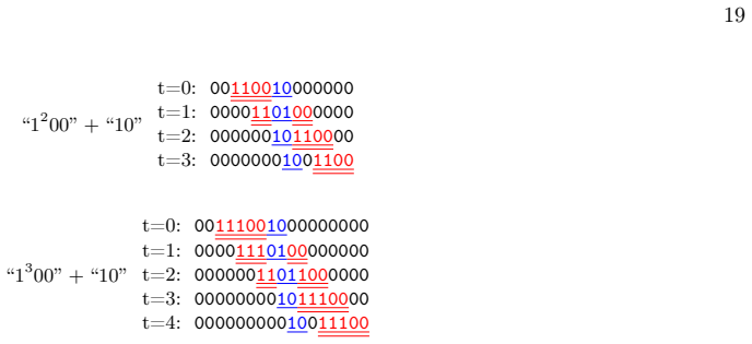
- Figure 12 (BBS-V(2) time evolution): The soliton decomposition is indicated by single, double, and triple underlining. The triple-underlining (red, 5-soliton) is mentioned in the caption but is difficult to distinguish from double-underlining in the figure. Consider using a more visually distinct marking (e.g., a different color or a labeled bracket above the soliton).
- Remark II.10: The configuration η defined in Eq. (52) is said to belong to Ω but not to Ω_{A_BBS}. The construction {η_n}_{n≥0} = 1^2 0 1^3 0^2 · · · 1^{k+1} 0^k · · · is clear, but the extension to the negative half-line (η_{−n} = η_{n−1}) should be more explicitly stated as producing a configuration in Ω (i.e., with arbitrarily long zero blocks in both directions).
- Table VII: The phase shift entry for BBS-V(2) lists Φ(γ_l, γ_m) = −m(1 + 2/l) for l > m ≥ 1. It would be helpful to also list the special case (l, m) = (2, 1) explicitly as Φ(γ_2, γ_1) = −1·(1+1) = −2 and Φ(γ_1, γ_2) = 2+2 = 4, to allow quick comparison with the examples in Figure 15.
- Section III.A: The description of BBS-S(2) states 'When the carrier picks up a ball, it moves two sites ahead and drops the ball there if the site is empty. Otherwise, it again moves two sites ahead and repeats the same procedure.' This is slightly ambiguous: does 'moves two sites ahead' mean skipping one site, or moving to the site two positions later? A diagram or a more precise formulation (e.g., 'advances by 2 positions') would help.
- Appendix B, proof of Remark III.2: The three cases for Q_{m_1−1} ∈ {q_0, q_1, q_2} are analyzed. For the case Q_{m_1−1} = q_0, the argument is that η_{m_1−1} must be 0, contradicting the minimality of m_1. This step could be made more explicit: why must η_{m_1−1} = 0 when Q_{m_1−1} = q_0?
- The paper uses both 'Bernoulli product measure' and 'Bernoulli distribution' somewhat interchangeably. Standardizing on one term throughout would improve readability.
- Reference [13] (Maeno, Tsujimoto, Yura, Physica D, 2025): Since this is the primary source for the three models, and the present paper builds directly on its classification results, the authors should verify that [13] is publicly available (or at least accessible to referees) at the time of submission, as the self-containedness of the present paper partially depends on it.
Circularity Check
No significant circularity found; the paper is self-contained mathematical derivation.
full rationale
The paper's central results (Theorems V.1 and V.2) are proved from first principles using the explicit Mealy automaton transition tables (Tables I–III) and the general invariance criteria (Theorems II.12 and II.13). The general criteria themselves are derived from the automaton axioms (A1)–(A3) and the Markov/Bernoulli measure structure, without invoking external unverified results. The phase shifts and soliton velocities (Section IV) are computed directly from the dynamics via case analysis on concrete configurations, not fitted to data. The only external dependency is on [13] (Maeno, Tsujimoto, Yura) for the classification of 2-letter, 3-state Mealy automata and the model definitions, but this citation provides the input models rather than a load-bearing theorem that would make the present results tautological. The proof of Theorem V.1 relies on an exhaustive case analysis (Tables VIII–XIII) that is verifiable from the transition table of BBS-C(2). The proof of Theorem V.2 uses the particle-preserving property (verified explicitly in Tables XIV–XV) and Theorem II.13, which is proved in-line. No step in the derivation chain reduces to its inputs by construction, and no self-citation chain forces the conclusion.
Axiom & Free-Parameter Ledger
free parameters (2)
- p
- r
axioms (4)
- domain assumption Condition (A1): The automaton is bijective.
- domain assumption Condition (A2): There exists a unique q* with (φ(q*,0), ψ(q*,0)) = (q*,0).
- domain assumption Condition (A3): There exists N such that scanning 0^N resets any state to q*.
- domain assumption Particle-preserving property (Definition II.1).
read the original abstract
We study invariant measures for soliton systems described by Mealy automata. Motivated by recently introduced soliton models associated with 2-letter, 3-state Mealy automata, we formulate the time evolution induced by Mealy automata on bi-infinite configuration spaces. We provide sufficient conditions for the invariance of Bernoulli product measures and derive a criterion for the invariance of two-sided space-homogeneous Markov distributions. We then apply these general results to three soliton models, which can be interpreted as variants of the box-ball system (BBS). For two of these models, BBS-S(2) and BBS-V(2), we prove that Bernoulli product measures are invariant. For the remaining model, BBS-C(2), we establish a more general result: the invariance of two-sided space-homogeneous Markov distributions, which include Bernoulli product measures as a special case. Furthermore, for all three models, we compute the phase shift associated with the interaction of two solitons, as well as the velocity of an isolated soliton. Although the latter has already been studied previously, both quantities constitute fundamental characteristics for understanding the generalized hydrodynamics of these systems. These results provide a foundation for the study of invariant measures, generalized Gibbs ensembles, and generalized hydrodynamic behavior in Mealy-automaton soliton systems.
Figures




Reference graph
Works this paper leans on
-
[1]
=r.(103) Case 1:˜ηends with˜ηn−1˜ηn = 12 (Table XI). TABLE XI. Transition probabilities and patterns (Case 1) Qn ηProbability/Common factor q0 · · ·100p(1−r) q1 · · ·110r(1−r) q2 · · ·111r 2 22 Case 2:˜ηends with˜ηn−1˜ηn = 01and when the carrier runs from right to left, it encounters“00”before“11”in˜η (Table XII). TABLE XII. Transition probabilities and p...
-
[2]
00”. However, the following examples in Figs. 16 and 17 illustrate that“00
=p(1−r) :r(1−r) :r 2. Substituting this constant ratio into (103) confirms the equality, which implies (101). B. Invariant Measures for BBS-S(2) and BBS-V(2) Theorem V.2.Forp, r∈(0,1),ν M is an invariant measure for the systemsBBS-S(2)andBBS-V(2)if and only if r= 1−p. This condition corresponds to the case whereνM is the Bernoulli product measureνp. Proof...
-
[3]
S. Novikov, S. V. Manakov, L. P. Pitaevskii, and V. E. Zakharov,Theory of solitons: the inverse scattering method (Springer, New York, 1984)
work page 1984
-
[4]
Walters,An introduction to ergodic theory, Vol
P. Walters,An introduction to ergodic theory, Vol. 79 (Springer, New York, 2000)
work page 2000
-
[5]
S. Friedli and Y. Velenik,Statistical mechanics of lattice systems: a concrete mathematical introduction(Cambridge Uni- versity Press, Cambridge, 2017)
work page 2017
-
[6]
H. Spohn, Generalized Gibbs ensembles of the classical Toda chain, Journal of Statistical Physics180, 4 (2020)
work page 2020
- [7]
-
[8]
B. Doyon, Generalized hydrodynamics of the classical Toda system, Journal of Mathematical Physics60, 073302 (2019)
work page 2019
-
[9]
D. Takahashi and J. Satsuma, A soliton cellular automaton, Journal of the Physical Society of Japan59, 3514 (1990)
work page 1990
-
[10]
D. Takahashi and J. Matsukidaira, Box and ball system with a carrier and ultradiscrete modified KdV equation, Journal of Physics A: Mathematical and General30, L733 (1997)
work page 1997
-
[11]
D. Croydon, T. Kato, M. Sasada, and S. Tsujimoto,Dynamics of the box-ball system with random initial conditions via Pitman ’s transformation, Vol. 283 (American Mathematical Society, Providence, RI, 2023)
work page 2023
-
[12]
P. A. Ferrari, C. Nguyen, L. T. Rolla, and M. Wang, Soliton decomposition of the box-ball system, Forum of Mathematics, Sigma9, e60 (2021)
work page 2021
-
[13]
D. A. Croydon and M. Sasada, Generalized hydrodynamic limit for the box–ball system, Communications in Mathematical Physics383, 427 (2021)
work page 2021
-
[14]
G. H. Mealy, A method for synthesizing sequential circuits, The Bell System Technical Journal34, 1045 (1955)
work page 1955
- [15]
discussion (0)
Sign in with ORCID, Apple, or X to comment. Anyone can read and Pith papers without signing in.