REVIEW 2 major objections 7 minor 59 references
Cut ResNet-50 compute nearly in half, gain 0.8% accuracy
Reviewed by Pith at T0; open to challenge. T0 means a machine referee read the full paper against a public rubric. the ladder, T0–T4 →
T0 review · glm-5.2
2026-07-09 22:10 UTC pith:C5DFR4Q2
load-bearing objection Solid engineering integration of known compression ideas; the compound shrinking estimator has an unvalidated gap but the empirical results stand on their own. the 2 major comments →
EdgeCompress: Coupling Multidimensional Model Compression and Dynamic Inference for EdgeAI
The pith
A machine-rendered reading of the paper's core claim, the machinery that carries it, and where it could break.
Core claim
The paper's load-bearing finding is that image-level spatial redundancy, architecture-level parameter redundancy, and instance-level difficulty redundancy are largely independent and can be stripped away in sequence without compounding accuracy loss. A 0.27-million-parameter foreground predictor replaces expensive gradient-based saliency with a fast bounding-box regression, enabling resolution reduction that preserves foreground detail. A polynomial accuracy estimator fit on separately-shrunk models then allocates a shrinking coefficient to each of the three architectural dimensions so that the dimension most sensitive to accuracy is shrunk least. Finally, a probability-difference confidence
What carries the argument
Three coupled mechanisms: (1) Dynamic Image Cropping (DIC) — a lightweight residual-bottleneck predictor trained on Grad-CAM-generated pseudo-bounding-boxes regresses foreground coordinates in 0.09B MACs, replacing the expensive backpropagation of Grad-CAM at inference time. (2) Compound Shrinking (CS) — a quadratic polynomial estimator approximates each dimension's accuracy-vs-MACs curve from a few sampled models, then a geometric-mean formula (Eq. 5) assigns a per-dimension shrinking coefficient inversely proportional to that dimension's accuracy drop, so the most accuracy-sensitive dimension is shrunk least. (3) Dynamic Inference (DI) — multiple compound-shrunk sub-networks are cascaded;
Load-bearing premise
The compound shrinking strategy assumes that a simple quadratic curve, fit by shrinking each network dimension in isolation, can predict how accuracy will behave when all three dimensions are shrunk simultaneously — it does not account for interaction effects between dimensions.
What would settle it
Train the compound-shrinking accuracy estimator on separately-shrunk models, then compare its predicted accuracy for a jointly-shrunk configuration against the actual measured accuracy of that jointly-shrunk model. If the gap exceeds the RMSE of ~1.7e-2 reported for the individual-dimension fits, the estimator is miscalibrated and the shrinking coefficients it produces are suboptimal.
If this is right
- Edge devices with heterogeneous power budgets could load only the subset of cascaded sub-networks that fits their current envelope, making the same trained model family portable across devices from microcontrollers to desktop GPUs.
- The foreground-predictor-as-preprocessor pattern could extend beyond classification to any vision task where background dominates the frame, such as video surveillance or autonomous driving perception.
- If the probability-difference confidence metric generalizes, it could replace the standard max-softmax confidence used in most early-exit and cascaded-inference systems, improving exit decisions across the dynamic-neural-network field.
- The compound-shrinking coefficient formula could be applied to newer architecture families (Vision Transformers, MLP-Mixers) that also have separable depth, width, and input-resolution dimensions.
Where Pith is reading between the lines
- The quadratic accuracy estimator that drives compound shrinking is trained only on models where each dimension is shrunk in isolation; if depth-width-resolution interactions are non-additive, the allocated coefficients would be miscalibrated and the joint model would underperform the estimator's prediction. The paper does not report validation accuracy of the estimator on jointly-shrunk configurat
- The dynamic-inference gains depend on the empirical distribution of image difficulty in ImageNet-1K, where most images are 'easy'; on datasets with a heavier tail of hard examples, the average-case latency advantage of early exit would shrink.
- The foreground predictor is trained on Grad-CAM saliency maps generated from a specific teacher network (ResNet-50); if the teacher's saliency differs systematically from the optimal crop for a different downstream architecture, the predictor's bounding boxes could be suboptimal for non-ResNet backbones.
Editorial analysis
A structured set of objections, weighed in public.
Referee Report
Summary. The manuscript proposes EdgeCompress, a three-stage CNN compression framework for edge deployment. Stage 1 (Dynamic Image Cropping, DIC) trains a lightweight foreground predictor (0.27M parameters) to crop informative regions, using Grad-CAM-generated bounding boxes as pseudo-labels. Stage 2 (Compound Shrinking, CS) jointly compresses depth, width, and resolution using dimension-wise shrinking coefficients derived from a polynomial accuracy estimator. Stage 3 (Dynamic Inference, DI) cascades sub-networks of increasing complexity and terminates when a confidence metric (probability difference between top-2 logits) exceeds a threshold, accumulating logits across models. Experiments on ImageNet-1K report 48.8% MACs reduction for ResNet-50 with +0.8% top-1 accuracy, and 4.1% accuracy improvement over HRank at similar computation. Code is publicly available.
Significance. The paper addresses a practically important problem—efficient CNN inference on resource-constrained edge devices—and combines input-level, architecture-level, and runtime-level compression in a unified pipeline. The public code release and reproducibility commitment are notable strengths. The experiments are extensive: four datasets, three hardware platforms (AGX Xavier, Jetson Nano, Intel CPU), multiple baselines, and an ablation study (Table XV). The lightweight foreground predictor design (Table XIV) and the probability-difference confidence metric (Table IV) are reasonable engineering contributions. The central empirical claim is supported by actually trained and evaluated models, not by estimator predictions alone.
major comments (2)
- §III.C, Eq. (5)–(6): The compound shrinking coefficients are derived from accuracy drops estimated by a quadratic polynomial (Eq. 6) fit only on models where each dimension is shrunk separately (Fig. 5). These coefficients then guide joint shrinking of all three dimensions. However, the estimator contains no interaction terms and the paper never reports its prediction error on jointly-shrunk configurations. If dimension interactions (e.g., width–resolution) are non-negligible, the computed coefficients may misallocate the shrinking budget, yielding suboptimal sub-networks. This concern is about pipeline optimality, not the correctness of the final reported numbers (which come from trained models). The authors should either (a) validate the estimator on jointly-shrunk configurations by reporting prediction error, or (b) discuss this limitation and justify why interaction effects are minor
- Fig. 13 caption: The foreground predictor is reported to achieve 62.1% mAP on ImageNet-1K validation, but the paper does not analyze how localization failures affect downstream classification accuracy. Since DIC is the first stage of the pipeline, systematic cropping errors on certain classes or image types could degrade classification. What happens when the predictor produces a poor bounding box—is there a fallback, or does classification accuracy degrade? A per-class or failure-case analysis, or at minimum a statement on robustness to predictor failures, would address this.
minor comments (7)
- Table III lists 6 sub-networks, but §IV.J.2 and Fig. 12 conclude that 2 models is optimal for dynamic inference. The paper should clarify whether the final reported results use 2 or 6 models, and if 2, explain why Table III presents a different configuration.
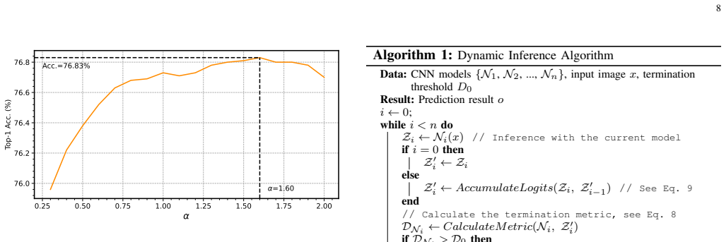
- §III.D.2, Eq. (9): The logit accumulation weight α=1.60 is selected empirically (Fig. 8). The search range and granularity for α are not specified. Stating these would help reproducibility.
- Table XV: EC-Dynamic reports lower latency (7.0 ms) than EC-Static (8.3 ms) at similar MACs (1.8B). While this is attributed to early-termination, the table would benefit from stating the average number of models activated per image to make the efficiency gain concrete.
- §IV.G.1: The comparison with SOTA methods (Fig. 11) aggregates results from different papers. The training settings (epochs, hyperparameters, data augmentation) for these baselines may differ. A note confirming comparable training protocols would make the comparison verifiable.
- The reference numbering in the bibliography appears inconsistent—several citation numbers in the text (e.g., [8], [10], [11], [12]–[16]) do not match the reference list entries. The authors should verify all citation numbers.
- §III.A: The salience threshold t=0.5 is selected from three values (Table I). A finer search or a brief justification for why only three values were tested would strengthen the claim that t=0.5 is near-optimal.
- Abstract and §IV.G: The claim of 4.1% improvement over HRank is a key headline result. The paper should note the publication year of HRank and whether more recent compression methods (2022–2023) have been considered as baselines, since the field moves quickly.
Circularity Check
No circularity found: EdgeCompress derivation chain is self-contained and empirically validated against external benchmarks
full rationale
The paper's derivation chain is self-contained and does not exhibit circular reasoning. The compound shrinking coefficients (Eq. 5) are computed from accuracy drops estimated by a polynomial estimator (Eq. 6) that is fitted to sampled data from separately-shrunk models (Fig. 5). While the reader correctly notes that this estimator lacks interaction terms for jointly-shrunk configurations, this is a modeling assumption and a correctness/optimality risk, not circularity: the estimator makes falsifiable predictions about unseen MACs regimes, and the final reported results (Table IX, Fig. 11) come from actually trained and evaluated models, not from the estimator's predictions. The confidence metric (Eq. 8) is a novel proposal validated against the standard 'highest probability' metric (Table IV, Fig. 7) using Wasserstein distance on sampled positive/negative predictions. The prediction accumulation (Eq. 9) is a logit-level operation with a hyperparameter α tuned empirically (Fig. 8). No step reduces to its inputs by definition, no 'prediction' is a fitted parameter renamed, and no self-citation chain forces the central result. The paper's claims are validated against external benchmarks (ImageNet-1K) and compared against independent SOTA methods (HRank, GAL-1, etc.), so the derivation is self-contained against external evidence.
Axiom & Free-Parameter Ledger
free parameters (5)
- t (salience threshold) =
0.5
- α (logit accumulation weight) =
1.60
- D0 (termination threshold) =
0.1–0.4 (multiple values)
- a_s, b_s (polynomial estimator coefficients) =
Fitted per dimension via least-squares (Fig. 5)
- Number of cascaded models =
2 (optimal)
axioms (4)
- domain assumption Grad-CAM salience maps accurately identify the foreground object region for bounding box generation.
- ad hoc to paper Accuracy as a function of MACs is well-approximated by a quadratic polynomial for each dimension independently.
- ad hoc to paper Dimension-wise accuracy drops are independent (no interaction effects between depth, width, and resolution shrinking).
- domain assumption The probability difference (top-1 minus top-2 softmax probability) is a reliable indicator of prediction correctness.
read the original abstract
Convolutional neural networks (CNNs) have demonstrated encouraging results in image classification tasks. However, the prohibitive computational cost of CNNs hinders the deployment of CNNs onto resource-constrained embedded devices. To address this issue, we propose EdgeCompress, a comprehensive compression framework to reduce the computational overhead of CNNs. In EdgeCompress, we first introduce dynamic image cropping (DIC), where we design a lightweight foreground predictor to accurately crop the most informative foreground object of input images for inference, which avoids redundant computation on background regions. Subsequently, we present compound shrinking (CS) to collaboratively compress the three dimensions (depth, width, and resolution) of CNNs according to their contribution to accuracy and model computation. DIC and CS together constitute a multidimensional CNN compression framework, which is able to comprehensively reduce the computational redundancy in both input images and neural network architectures, thereby improving the inference efficiency of CNNs. Further, we present a dynamic inference framework to efficiently process input images with different recognition difficulties, where we cascade multiple models with different complexities from our compression framework and dynamically adopt different models for different input images, which further compresses the computational redundancy and improves the inference efficiency of CNNs, facilitating the deployment of advanced CNNs onto embedded hardware. Experiments on ImageNet-1K demonstrate that EdgeCompress reduces the computation of ResNet-50 by 48.8% while improving the top-1 accuracy by 0.8%. Meanwhile, we improve the accuracy by 4.1% with similar computation compared to HRank, the state-of-the-art compression framework. The source code and models are available at https://github.com/ntuliuteam/edge-compress
Figures




Reference graph
Works this paper leans on
-
[1]
Imagenet: A large-scale hierarchical image database,
J. Denget al., “Imagenet: A large-scale hierarchical image database,” inCVPR, 2009
work page 2009
-
[2]
Microsoft coco: Common objects in context,
T.-Y . Linet al., “Microsoft coco: Common objects in context,” inECCV, 2014
work page 2014
-
[3]
Efficientnet: Rethinking model scaling for convo- lutional neural networks,
M. Tan and Q. Le, “Efficientnet: Rethinking model scaling for convo- lutional neural networks,” inICML, 2019
work page 2019
-
[4]
Designing network design spaces,
I. Radosavovicet al., “Designing network design spaces,” inCVPR, 2020
work page 2020
- [5]
-
[6]
Edge computing: Vision and challenges,
W. Shiet al., “Edge computing: Vision and challenges,”IoT Journal, 2016
work page 2016
-
[7]
Update compression for deep neural networks on the edge,
B. Chenet al., “Update compression for deep neural networks on the edge,” inCVPR Workshops, 2022
work page 2022
-
[8]
Mobilenetv2: Inverted residuals and linear bottle- necks,
M. Sandleret al., “Mobilenetv2: Inverted residuals and linear bottle- necks,” inCVPR, 2018
work page 2018
-
[9]
Mnasnet: Platform-aware neural architecture search for mobile,
M. Tanet al., “Mnasnet: Platform-aware neural architecture search for mobile,” inCVPR, 2019
work page 2019
-
[10]
M. Zhuet al., “Dynamic resolution network,” inNeurIPS, 2021
work page 2021
-
[11]
Hrank: Filter pruning using high-rank feature map,
M. Linet al., “Hrank: Filter pruning using high-rank feature map,” in CVPR, 2020
work page 2020
-
[12]
Convolutional neural network pruning with structural redundancy reduction,
Z. Wanget al., “Convolutional neural network pruning with structural redundancy reduction,” inCVPR, 2021
work page 2021
- [13]
-
[14]
Importance estimation for neural network pruning,
P. Molchanovet al., “Importance estimation for neural network pruning,” inCVPR, 2019
work page 2019
-
[15]
DBP: Discrimination Based Block-Level Pruning for Deep Model Acceleration
W. Wanget al., “Dbp: Discrimination based block-level pruning for deep model acceleration,”arXiv preprint arXiv:1912.10178, 2019
work page internal anchor Pith review Pith/arXiv arXiv 1912
-
[16]
Decore: Deep compression with reinforcement learning,
M. Alwaniet al., “Decore: Deep compression with reinforcement learning,” inCVPR, 2022
work page 2022
-
[17]
Glance and focus: A dynamic approach to reducing spatial redundancy in image classification,
Y . Wanget al., “Glance and focus: A dynamic approach to reducing spatial redundancy in image classification,” inNeurIPS, 2020
work page 2020
-
[18]
YOLOv4: Optimal Speed and Accuracy of Object Detection
A. Bochkovskiyet al., “Yolov4: Optimal speed and accuracy of object detection,”arXiv preprint arXiv:2004.10934, 2020
work page internal anchor Pith review Pith/arXiv arXiv 2004
-
[19]
Ssd: Single shot multibox detector,
W. Liuet al., “Ssd: Single shot multibox detector,” inECCV, 2016
work page 2016
-
[20]
Faster r-cnn: Towards real-time object detection with region proposal networks,
S. Renet al., “Faster r-cnn: Towards real-time object detection with region proposal networks,” inNeurIPS, 2015
work page 2015
- [21]
-
[22]
The pascal visual object classes (voc) challenge,
M. Everinghamet al., “The pascal visual object classes (voc) challenge,” IJCV, 2010
work page 2010
-
[23]
Unsupervised object discovery and co-localization by deep descriptor transformation,
X.-S. Weiet al., “Unsupervised object discovery and co-localization by deep descriptor transformation,”Pattern Recognition, 2019
work page 2019
-
[24]
Rethinking the route towards weakly supervised object localization,
C.-L. Zhanget al., “Rethinking the route towards weakly supervised object localization,” inCVPR, 2020
work page 2020
-
[25]
Learning deep features for discriminative localization,
B. Zhouet al., “Learning deep features for discriminative localization,” inCVPR, 2016
work page 2016
-
[26]
Grad-cam: Visual explanations from deep networks via gradient-based localization,
R. R. Selvarajuet al., “Grad-cam: Visual explanations from deep networks via gradient-based localization,” inCVPR, 2017
work page 2017
-
[27]
Adversarial complementary learning for weakly supervised object localization,
X. Zhanget al., “Adversarial complementary learning for weakly supervised object localization,” inCVPR, 2018
work page 2018
-
[28]
Bringing ai to edge: From deep learning’s perspective,
D. Liuet al., “Bringing ai to edge: From deep learning’s perspective,” Neurocomputing, 2022
work page 2022
-
[29]
Layer pruning for obtaining shallower resnets,
K. Zhang and G. Liu, “Layer pruning for obtaining shallower resnets,” IEEE Signal Processing Letters, 2022
work page 2022
-
[30]
Branchynet: Fast inference via early exiting from deep neural networks,
S. Teerapittayanonet al., “Branchynet: Fast inference via early exiting from deep neural networks,” inICPR, 2016
work page 2016
-
[31]
Multi-scale dense networks for resource efficient image classification,
G. Huanget al., “Multi-scale dense networks for resource efficient image classification,” inICLR, 2018
work page 2018
-
[32]
Adaptive neural networks for efficient inference,
T. Bolukbasiet al., “Adaptive neural networks for efficient inference,” inICML, 2017. 14
work page 2017
-
[33]
Adaptive Computation Time for Recurrent Neural Networks
A. Graves, “Adaptive computation time for recurrent neural networks,” arXiv preprint arXiv:1603.08983, 2016
work page internal anchor Pith review Pith/arXiv arXiv 2016
-
[34]
Skipnet: Learning dynamic routing in convolutional networks,
X. Wanget al., “Skipnet: Learning dynamic routing in convolutional networks,” inECCV, 2018
work page 2018
-
[35]
Convolutional networks with adaptive infer- ence graphs,
A. Veit and S. Belongie, “Convolutional networks with adaptive infer- ence graphs,” inECCV, 2018
work page 2018
-
[36]
Channel gating neural networks,
W. Huaet al., “Channel gating neural networks,”NeurIPS, 2019
work page 2019
- [37]
-
[38]
Dynamic channel pruning: Feature boosting and sup- pression,
X. Gaoet al., “Dynamic channel pruning: Feature boosting and sup- pression,” inICLR, 2019
work page 2019
-
[39]
Channel selection using gumbel softmax,
C. Herrmannet al., “Channel selection using gumbel softmax,” inECCV, 2020
work page 2020
-
[40]
Resolution adaptive networks for efficient inference,
L. Yanget al., “Resolution adaptive networks for efficient inference,” inCVPR, 2020
work page 2020
-
[41]
Deep residual learning for image recognition,
K. Heet al., “Deep residual learning for image recognition,” inCVPR, 2016
work page 2016
-
[42]
Tiny-dsod: Lightweight object detection for resource- restricted usages,
Y . Liet al., “Tiny-dsod: Lightweight object detection for resource- restricted usages,” inBMVC, 2018
work page 2018
-
[43]
Adam: A method for stochastic optimization,
D. P. Kingma and J. Ba, “Adam: A method for stochastic optimization,” inICLR, 2015
work page 2015
-
[44]
An exponential learning rate schedule for deep learning,
Z. Li and S. Arora, “An exponential learning rate schedule for deep learning,” inICLR, 2020
work page 2020
-
[45]
Hapi: Hardware-aware progressive inference,
S. Laskaridiset al., “Hapi: Hardware-aware progressive inference,” in ICCAD, 2020
work page 2020
-
[46]
Shallow-deep networks: Understanding and mitigating network overthinking,
Y . Kayaet al., “Shallow-deep networks: Understanding and mitigating network overthinking,” inICML, 2019
work page 2019
-
[47]
Very Deep Convolutional Networks for Large-Scale Image Recognition
K. Simonyan and A. Zisserman, “Very deep convolutional networks for large-scale image recognition,”arXiv preprint arXiv:1409.1556, 2014
work page internal anchor Pith review Pith/arXiv arXiv 2014
-
[48]
Rethinking the inception architecture for computer vision,
C. Szegedyet al., “Rethinking the inception architecture for computer vision,” inCVPR, 2016
work page 2016
-
[49]
S. Zagoruyko and N. Komodakis, “Wide residual networks,” inBMVC, 2016
work page 2016
-
[50]
Data-driven sparse structure selection for deep neural networks,
Z. Huang and N. Wang, “Data-driven sparse structure selection for deep neural networks,” inECCV, 2018
work page 2018
-
[51]
Learning versatile filters for efficient convolutional neural networks,
Y . Wanget al., “Learning versatile filters for efficient convolutional neural networks,” inNeurIPS, 2018
work page 2018
-
[52]
Provable filter pruning for efficient neural networks,
L. Liebenweinet al., “Provable filter pruning for efficient neural networks,” inICLR, 2019
work page 2019
-
[53]
Centripetal sgd for pruning very deep convolutional networks with complicated structure,
X. Dinget al., “Centripetal sgd for pruning very deep convolutional networks with complicated structure,” inCVPR, 2019
work page 2019
-
[54]
Towards optimal structured cnn pruning via generative adversarial learning,
S. Linet al., “Towards optimal structured cnn pruning via generative adversarial learning,” inCVPR, 2019
work page 2019
-
[55]
Autopruner: An end-to-end trainable filter pruning method for efficient deep model inference,
J.-H. Luo and J. Wu, “Autopruner: An end-to-end trainable filter pruning method for efficient deep model inference,”Pattern Recognition, 2020
work page 2020
-
[56]
Densely connected convolutional networks,
G. Huanget al., “Densely connected convolutional networks,” inCVPR, 2017
work page 2017
-
[57]
Batch normalization: Accelerating deep network training by reducing internal covariate shift,
S. Ioffe and C. Szegedy, “Batch normalization: Accelerating deep network training by reducing internal covariate shift,” inICML, 2015
work page 2015
-
[58]
Variational convolutional neural network pruning,
C. Zhaoet al., “Variational convolutional neural network pruning,” in CVPR, 2019. Hao Kongreceived the B.E. degree from University of Electronic Science and Technology of China, China, in 2019. He is currently a Ph.D. student at the School of Computer Science and Engineer- ing, Nanyang Technological University, Singapore. His research interests include ed...
work page 2019
-
[59]
He is currently pursuing the Ph.D degree from the School of Computer Science and Engineering at Nanyang Technological University, Singapore. His current research interests include edge intelli- gence, hardware-aware neural architecture search, and model compression. Ravi Subramaniamis a Distinguished Technologist at HP Inc working on Machine Learning algo...
work page 2007
discussion (0)
Sign in with ORCID, Apple, or X to comment. Anyone can read and Pith papers without signing in.